

Charles Cox Zac Clausing
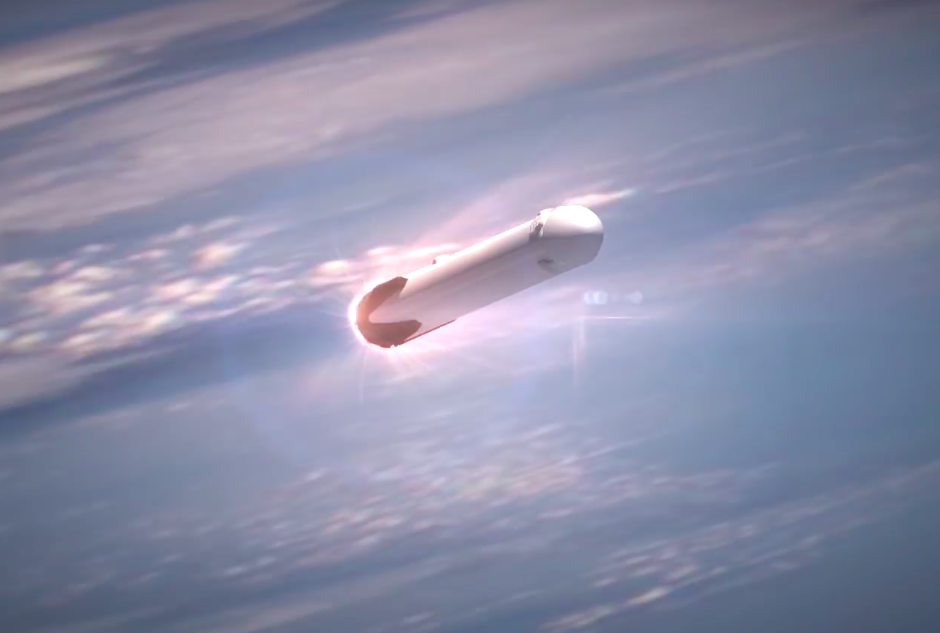
Falcon 9 Re-entry Burn
Thrust Vector Control of a Hypersonic Re-entry Vehicle
Project team member(s): Charles Cox, Zac Clausing
Abstract
A controller for managing the atmosheric re-entry orientation (1-DOF) of a hypersonic vehicle with a high length to diameter ratio will be developed and investigated. This model will approximate the conditions experienced by a SpaceX Falcon 9 first stage executing a re-entry burn in preparation for a propulsive landing. The vehicle is assumed to operate at high altitude in a free molecular flow field, such that the aerodynamic forces acting on the body can be readily determined. The plant will be modeled as an inverted pendulum, with four relevant forces acting on the vehicle: gravity, thrust, lift, and drag. A proportional-integral-differential (PID) controller will then be incorporated in a unity gain negative feedback configuration to alter the response characteristics of the system. Comparisons will be made between a linearized plant model and several nonlinear configurations.
Advanced Feature:
A Simulink model will be developed to investigate the fully non-linear nature of the system. A simple linearized model will also be analyzed using a variety of hand calculations, and the results from the two cases will be compared.
Introduction
Propulsive re-entry and landing techniques are increasingly relevant to the economics of spaceflight and will serve as a key enabling technology for ambitious extraterrestrial exploration efforts in the future. By analyzing a highly simplified one degree of freedom system, it is hoped that insights will be gained which are applicable to more realistic flight vehicles requiring robust control in six degrees of freedom (3 rotational and 3 translational modes). Experience gained developing Simulink models for highly non-linear systems will be of particular value.
Plant Model
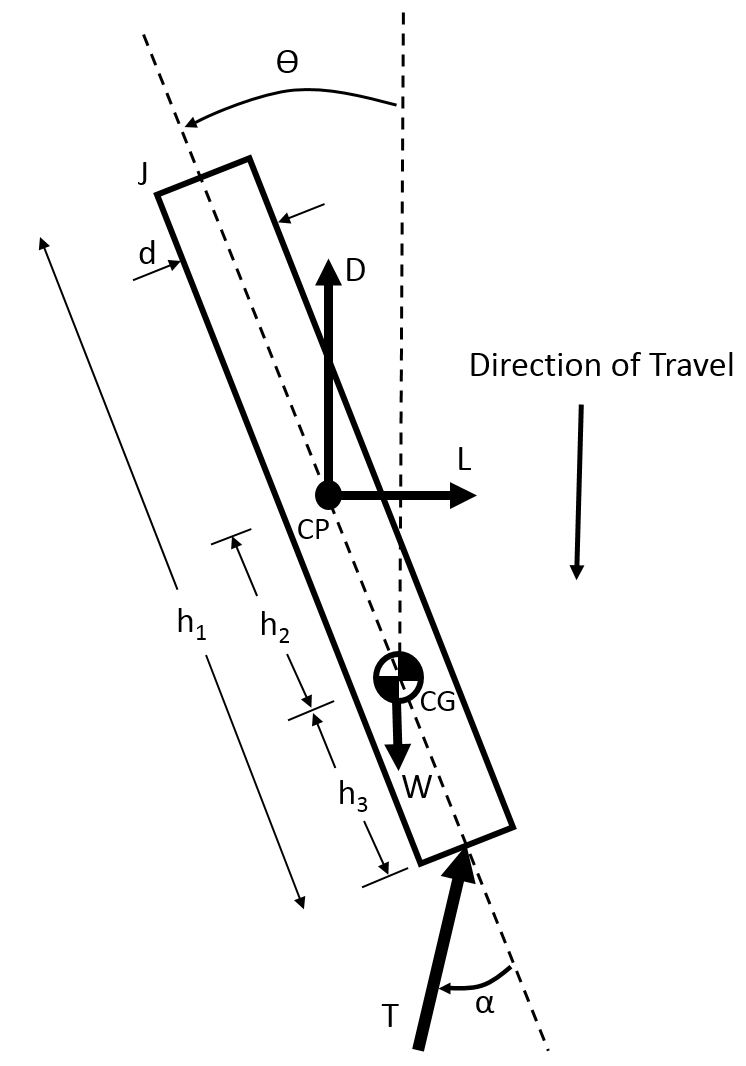
The descending rocket is modeled as a rigid cylindrical rod, rotating freely about its center of mass in response to torques generated by aerodynamic and thrust forces. The output parameter of interest is the angle theta, or the angle of the rocket with respect to vertical. The angle of the thrust force with respect to the vehicle centerline, alpha, will be taken as the plant input parameter and will be used to control the attitude of the rocket. A free body diagram for the system is shown below:
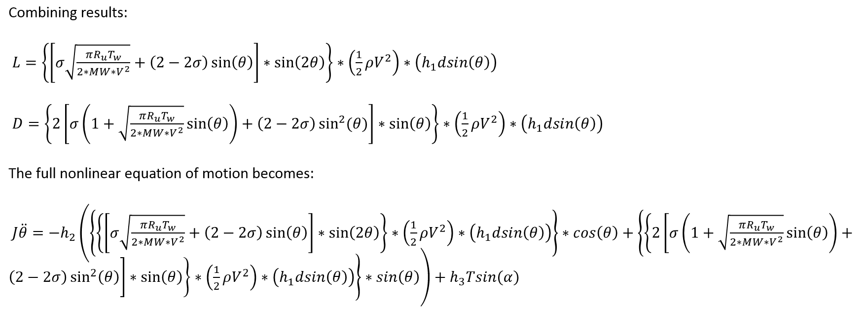
The approximate nonlinear equation of motion for the plant is:

Assuming that the vehicle angle theta remains small, we can neglect the theta^2 term to arrive at a simple linear system:
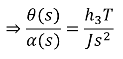
This system can be represented as a transfer function in the Laplace domain, as shown below:

The equation of motion for the plant is derived by considering the summation of moments about the rocket's center of gravity. The lift and drag forces are estimated as those acting on a flat plate in free molecular flow at an angle of attack theta. The derivation proceeds as follows:

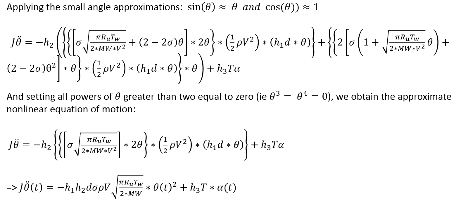
If we further assume that the theta^2 term is approximately equal to zero, the system becomes linear and we can form a transfer function, as shown below:
For the purposes of this project, all parameters except theta and alpha will be assumed constant. The parameters of interest are listed below along with their estimated values.
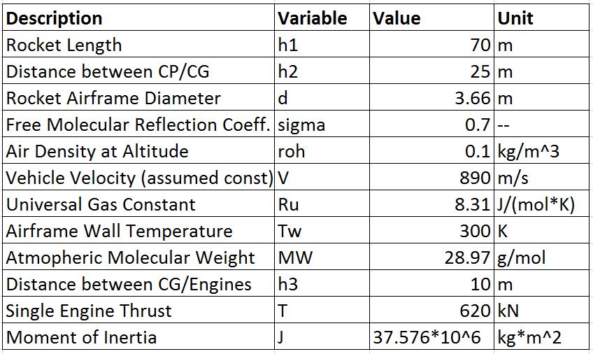
The values presented above are based on the approximate mass and dimensions of the Falcon 9 first stage, obtained from publicly available sources.
System Models
Three separate plant models will be considered during the course of this project. The first is the fully linear system presented above:
The second system is the approximate nonlinear equation of motion, which will be referenced as "nonlinear case 1":
And the third is this nonlinear system where the small angle approximation has been used to simplify only the cosine terms, and the sine terms are left intact. This will be termed "nonlinear case 2":

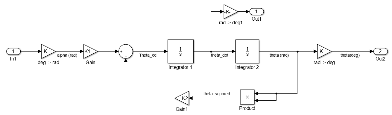
Both nonlinear plants will be implemented in Simulink, and their behavior compared. The Simulink model for the first nonlinear case is attached below for reference. Additional details and models can be found in the "Files" section at the end of this document.
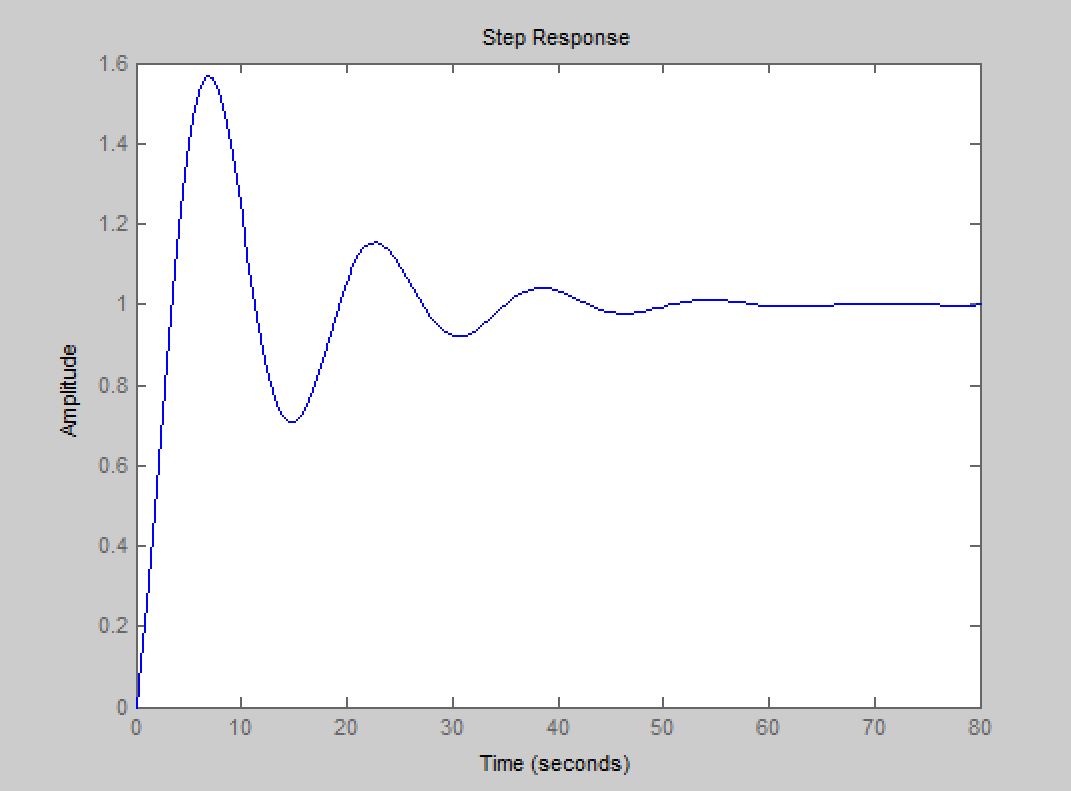
To confirm that our plant model accurately represents the physical system, we input a unit step into the open loop linearized plant, and examine the system response:

The temporal response of this system makes sense given our physical intuition of how the plant should work. A step change in the angle (alpha) of the thrust vector will effectively cause the rocket to rotate, with the angle theta increasing at an increasing rate, as observed in the plot above. This confirms that the plant model is capturing at least the most basic properties of the physical system, and provides confidence to begin designing a controller.
Control Design
The purpose of the controller is to ensure that the re-entry angle (theta) of the vehicle can be set to a desired value from approximately -15 degrees to +15 degrees, and the vehicle will maintain this angle over time, thus completing a successful reentry. The controller must take in a desired angle (theta_desired), and output a command thrust vector control (TVC) angle alpha. This TVC angle will then be fed into the plant model G(s) as described in the preceding section.
Key design objectives for the closed loop system response include:
 I.   Reasonably "fast" response:  it is desired that the vehicle will reach the desired angle from
      -15 degrees to 15 degrees in 60 seconds or less starting at theta = 0 degrees.

 II.   Minimal overshoot:  The vehicle angle theta must remain within the range from
       -20 to +20 degrees at all times.

 III.  Zero steady state error in response to a step input.

 IV.   Limited rotation rate. The vehicle can only withstand a certain angular velocity due to the resultant
       centripetal acceleration.  It is estimated that the maximum rotation rate is 8 degrees/second due to structural
       limitations, and therefore the rotation rate must not exceed this value at any time.  This will require balancing
       with Objective I.
To achieve these four distinct goals, a three term controller will be required. For initial control system design, we choose to implement a proportional-integral-derivative (PID) controller. Such a controller can be written in the form:

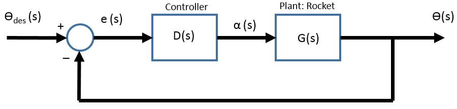
Where the constants Kp, Kd, and Ki are variables which can be used to tune the response of the closed loop system. The controller is placed in a negative feedback loop configuration, as shown below:
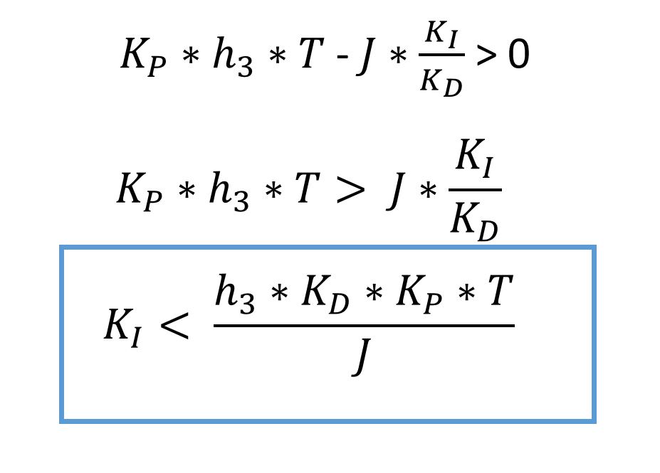
A Routh Array of the linearized model with PID control demonstrated that if Ki is set to 0, any positive values of Kp and Kd will ensure system stability. However, it also shows that adding a positive Ki can force the system to go unstable. The stability criterion for Ki is shown below here:
We will test this analysis with the linearized model's step response.
With a positive Kp and Kd, and Ki = 0, we were able to elicit a stable, sinusoidal response from the system as predicted. See plot below for Kd = 3, Kp = 5:
By increasing Kd to 10, it is possible to overdamp the system and reign in the overshoot and response time.

In addition, we tested implementing a Ki higher than the threshold predicted for stability by the Routh Array. With the threshold coming to 2.6 for Kp = 5 and Kd = 3, we set Ki equal to 3. The response was unstable, as predicted:

Starting with these gain values (Kp = 5, Kd = 3, and Ki chosen to ensure stability), we'll next implement a PID controller in Simulink with the full nonlinear plant and compare the results.
Results
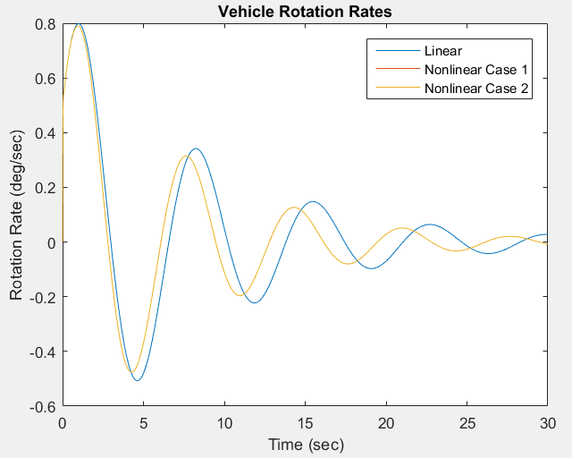
Using the values of Kp = 5 and Kd = 3 that were determined to produce a desirable damped step response for the linear system, and setting Ki to 1/2 the value predicted to cause instability using Routh's stability criterion (ie, setting Ki = 1.2375), the nonlinear models were implemented in Simulink and given a unit step input. The plot below shows a comparison between the closed loop response of the fully linear system, and the two nonlinear models.

It is noted that the response of both nonlinear systems is virtually identical, as would be expected for small theta. Interestingly, while the response of the linear and nonlinear systems is qualitatively similar, there are substantial differences in both the maximum overshoot and frequency of oscillation. The nonlinear system experiences somewhat lower maximum overshoot, which results from the presence of aerodynamic forces acting on the vehicle to oppose it's rotation, as would be expected.
Next, the rotation rates for the vehicle were determined, and are presented below:
The maximum rotation rate in response to a unit step input is approximately 0.8 degrees per second, well below the maximum threshold of 8 deg/second which was determined due to the structural limitations of the vehicle.
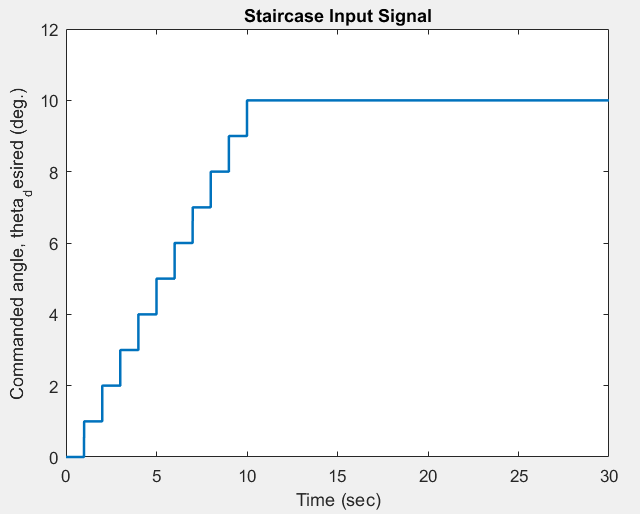
To demonstrate that the closed loop system response is desirable for a more representative input case, a series of 10 distinct one degree step inputs were provided to the vehicle at 1 second intervals, forming a "staircase" input signal. In effect, this signal could be used to command the rocket from a 0 to 10 degree angle of attack. The input signal is provided below for reference.
The response of the first nonlinear system to the staircase input is shown below.
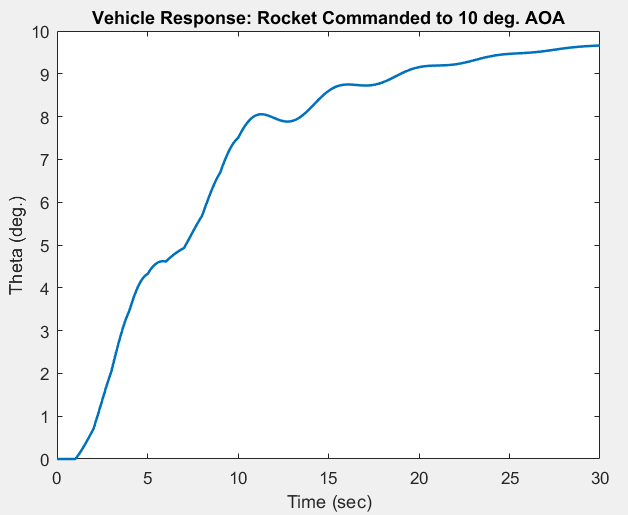
Overall, it seems that the closed loop system response is as desired. The vehicle angle theta tracks the input signal reasonably well, and approaches the commanded value of 10 degrees over time. However, one challenge noted with the step input approach is that the thrust vector control (TVC) angle alpha spikes to unrealistically high values in response to each step. A plot of this phenomenon for the staircase input is given below.

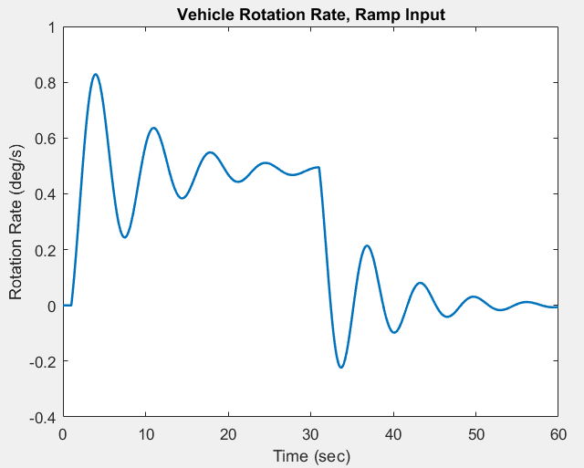
Realistic values for the TVC angle might range from approximately -20 degrees to 20 degrees at a maximum. Therefore, it is clear that the system response presented above for a staircase input could never be achieved. In an attempt to overcome this challenge, a ramp input was provided to the system instead. The input and resulting system response are shown below.

As the plot above shows, the closed loop system tracks the input signal quite well, reaching the targeted 15 degree angle of attack in approximately 45 seconds with zero steady state error and minimal overshoot. The maximum rotation rate for the vehicle with the ramp input is as follows:
And the thrust vector control angle now lies within reasonable limits:

Therefore, it is clear that the controller meets all design objectives when a ramp input signal is employed, providing rapid vehicle response, minimal overshoot, zero steady state error, reasonable rotation rates, and achievable TVC angles.
Conclusions
Our first conclusion is that the linearized model of the plant is actually fairly representative of the behavior of the nonlinear plant at high altitudes. This is due to two primary effects:
1) The angle of theta is small, so higher order terms of theta (and even first order terms) have a minimal impact on the system behavior. This is true across all altitude profiles.
2) More importantly, the terms dependent on theta are aerodynamic terms, and at high operating altitudes, the air is extremely thin (represented as very low density). With so little air, aerodynamic effects become very small in comparison to the thrust of a Merlin 1D engine.
As altitude decreases and density increases, the aerodynamic nonlinearities of the system grow, creating greater and greater divergence between the linear and non-linear models.
A second conclusion is that there exists a stark tension between a "fast" response time, and making sure the rocket doesn't tear itself apart as it rotates. While rotating 15 degrees in 30 seconds doesn't seem like a big deal, the scale of the system really amplifies the effects of that rotation. We are essentially spinning a 14 story building. The centripetal acceleration at points far from the center of rotation (for example, the engines), can become quite large. Ensuring that those forces don't become too large is an extremely important exercise that serves as a primary system limiter.
A final conclusion is that a step input to the system is not realistic; in practice, you would feed the system controlled ramp inputs, as demonstrated in the results section above. This simple change has a dramatic impact on the controller effort (TVC angle) required by the system, and on the peak vehicle rotation rates.
If we had more time, we would like to look at constraining the system even further to increase its realism. For example, limiting the rate of change of the thrust vector angle to represent the capabilitiies of the engine actuators (as opposed to just the vehicle body, as we did) would be very interesting and worthwhile. Another improvement would be adding in the time delay that's incurred by processing time + signal travel time + implementation by physical actuators. A sensor model could also be developed and incorporated into the closed loop system to account for the dynamics of accelerometers and similar instrumentation used to measure the vehicle rotation rate.
Overall, we were pleased with the outcome of this control design exercise. We achieved all of the initial design objectives, and gained valuable experience and intuition modeling nonlinear systems. Propulsive re-entry really is a very challenging problem with several layers of complexity, so getting as far as we did within the constraints of E105 tools and time limitations should be deemed a success.
Acknowledgments
We would like to thank SpaceX for publishing so many key details about the Falcon 9. The availability of data makes it much easier to perform this type of analysis. Thanks also to the E105 teaching team for their support and guidance.
Files
The code attached below contains the analysis of the linearized plant model -- both open loop and closed loop PID. Attach:cox_linearmodel_matlab
The following code defines parameters of interest for use in Simulink, and plots Simulink results. Note that in order to return the desired results, the "simulink_model_inputs" code must be run first, followed by the "simulink_model" file attached below. Finally, running "simulink_model_inputs" again will generate the appropriate plots. Attach:Clausing_simulink_model_inputs
The Simulink model used to investigate the nonlinear rocket plant is provided below. Attach:Clausing_simulink_model
References
Storch, J.A., "Aerodynamic Disturbances on Spacecraft in Free-Molecular Flow", The Aerospace Corporation, El Segundo, CA, Published 17 October, 2002.
SpaceX, St. "SpaceX Falcon 9 User's Guide." PAYLOAD USER'S GUIDE (n.d.): n. pag. SpaceX.com. Web. 2016.