

Alexa Siu Jonah Kohen

PID Control of an Autonomous Two-Degree-of-Freedom Robotic Arm
Project team members: Alexa Siu & Jonah Kohen
Abstract
Robot-assisted minimally invasive surgery has many advantages over traditional open surgery. Current robotic systems are teleoperated by a human operator, however, there has been recent work on autonomous robot agents that can assist the surgeon in subtasks. Such agent would allow the surgeon to concentrate his/her efforts on the more critical/complex parts of the surgery. The robot's predefined tasks could be as simple as making an incision along a path. In this work, we model a 2-degree-of-freedom (DOF) planar link robotic arm with revolute joints and propose control of its end-effector trajectory along a path. First, we derived the kinematics and dynamics equations governing the robotic arm's motion and planed for the desired paths. Our plant in this system was the robotic arm, where its inputs are torque at each joint and output are the angles at each joint. Second, we implemented a controller for the closed-loop system (without disturbances) and evaluated its performance in Simulink. In the closed-loop system, our input were the desired angles, and our output were the actual angles. Our main control goal was to achieve good reference tracking with as little overshoot and oscillations. If this were in a clinical scenario, where the robotic arm was tracing a path along a delicate area, any overshoot and oscillations could be dangerous. We implemented a separate PID controller for each joint and tuned the gains for a step-reference input. In both controllers, the most we could achieve was ~15% overshoot, therefore we optimized for minimal settling time and steady state error. Lastly, we evaluated how well our system was at reference tracking when we input our desired paths. Our output angles varied very little from the desired angles so we were able to achieve our main goal. However at the initial time, we have a large overshoot that deviates from the desired path. Other limitations in our model are that our controller assumes independent joints and some environmental disturbances such as movements and sensor noise were not considered. Future work would aim to bring our model closer to reality by considering a 2-input PID controller and modeling of environmental disturbances.
Advanced Feature: a transfer function of fourth order or higher, simulink model of the nonlinear system
Introduction
Robot-assisted minimally invasive surgery has many advantages over traditional open surgery. Current robotic systems are teleoperated by a human operator. Given recent advances in computer vision and artificial intelligence, it would be interesting for the robot to be an autonomous agent assisting the surgeon in subtasks.This would allow the surgeon to concentrate his/her efforts on the more critical/complex parts of the surgery which would reduce surgeon fatigue, operation time, among others. The robot's predefined tasks could be as simple as making an incision along a path. Related research work includes the Human-Machine Collaborative system which is able to learn how to collaboratively assist the surgeon during a teleoperated task [1]. Having a predefined incision path, we propose position control of a 2 degree-of-freedom robotic arm to trace this path. Our system controller would aim to minimize any oscillations of the robot end-effector from the desired path. We will model the robotic arm as 2 linkages with revolute joints where we want to command joint torques to reach the desired position at each point along the path. We assume each joint, has sensors such as encoders that allow us to know the robotic arm's position and track the error.
Plant Model
Part 1: System Model
We model the robotic arm (our plant) as two linkages with revolute joints at Ao and Bo (Figure 1). Link A is attached to a Newtonian reference frame and has length LA. Link B is in contact with A through Bo and has length LB.

Figure 1:
Diagram of the robotic arm modeled as two linkages connected by revolute joints.
We can command torque to each motor joint to achieve the desired qA and qB. We also assume that the arm moves at a constant velocity, we assume frictionless joints and that at each joint we have encoders that allow us to monitor the arm's position. At each time step we want the end effector (point BE) to be at a certain x and y position.
The parameters and values relevant to this system are:
LA = 2.0 * 0.0254; % length of link A [m]
LB = 1.5 * 0.0254; % length of link B [m]
mA = 2; % mass of link A [kg]
mB = 1; % mass of link B [kg]
g = 9.81; % gravity [m/s^2]
We approximated these parameters from measuring a surgical tool.
Part 2: Path Planning (Kinematics Equations)
With the simplified model described previously, we derive the governing kinematic equations.
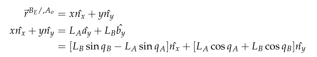
Taking the dot product with nx and ny, we obtain our final equations of motion:
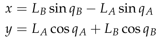
With these two equations we can determine the necessary qA and qB to achieve a certain path in x, y (cartesian coordinates). We experimented with two paths: 1) a straight line path and 2) a sinusoidal path. The results are shown below.

Figure 2:
Straight Line Path

Figure 3:
Sinusoidal Path
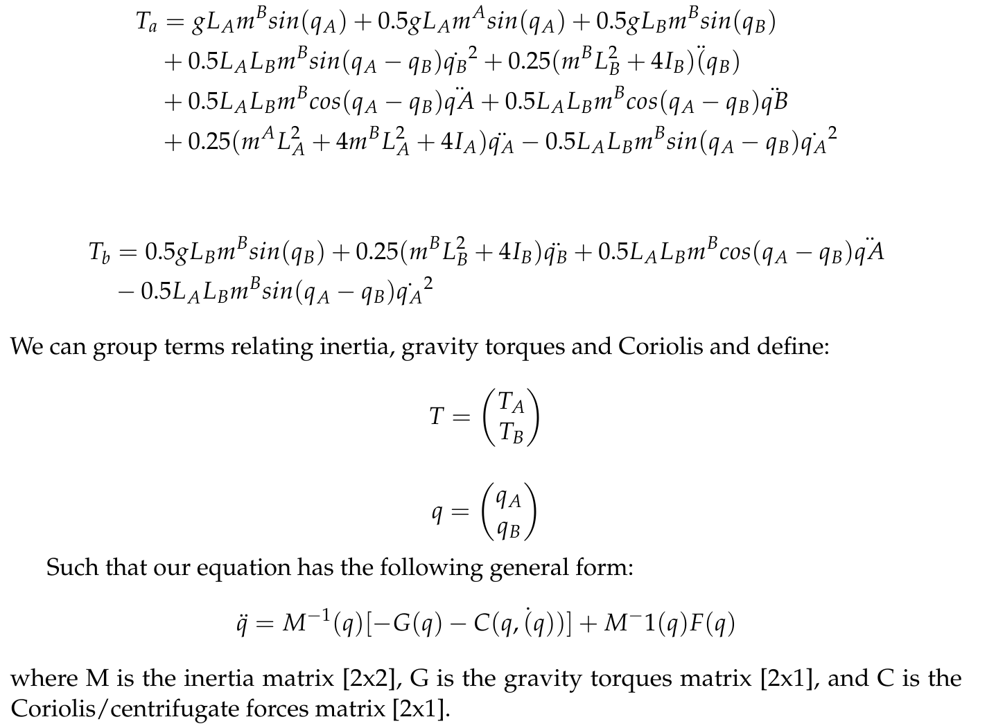
Part 3: Dynamics Equations
For deriving the dynamics equations, we used MotionGenesis (http://www.motiongenesis.com/) software. Detailed code and outputs can be found here: Attach:MG-code.zip. The resulting equations relating torques at each joint and angles are as follows:
Part 4: Block Diagram in Simulink and Open-Loop Behavior
Based on our dynamic equations, we will set torques at each joint as our plant input and joint angles as our plant output. With our kinematic equations, we can always relate these joint angles back to our desired end-effector position x, y (in cartesian coordinates).

The nonlinear equations were put into Simulink. A screenshot is shown below:

Figure 4 shows preliminary results from a simulation on the open loop system. The input for this experiment was a step (in torque) and the output signals were the joint angles (qA and qB). For Joint A, the output constant. However, for Joint B, the output grows to infinity which is neither desirable nor physically possible for our robotic arm.
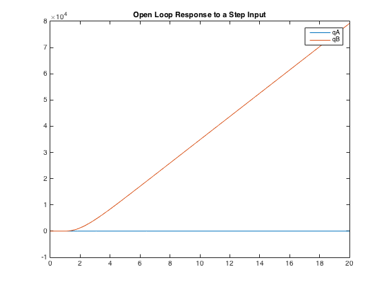
Figure 4:
Open Loop Response to a Step Input
Control Design
We wanted our controller to minimize overshoot, steady state error, and oscillation. In a surgical context, having a robot that initially overshoots how deep or how far it has to cut, coupled with a steady state error that guarantees an inaccurate incision depth, is unacceptable for precision surgery. Small amounts of oscillation in the arm's position, even for a few short moments, can lead to scarring and damage to healthy tissue. Reduction in all three of these error terms required the use of a PID controller. To minimize the steady-state error, we used integral control. Derivative control was added in order to minimize the overshoot and the additional oscillation brought upon by the integral controller.
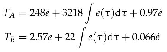
Using our previous notation from the Plant Model section and defining e as the error, i.e. e = qdesired - qactual, our controller equations are as follows:
A simplified block diagram and Simulink block diagram for the closed-loop system are in Figures 5 and 6.
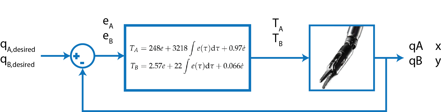
Figure 5:
Closed-Loop System Block Diagram

Figure 6:
Closed-Loop System Simulink Block Diagram
We implemented a PID controller for each joint angle, as can be seen from the block diagram (Figure 6). There are myriad limitations to the analysis we can do, given the nonlinearity and immense complexity of our system. First, we almost assume the joints are decoupled, while in reality when link A moves, the position of link B also changes. Our analysis is also hampered by the loss of our linear models. Throughout the course we have focused on developing controllers for linear systems. The heavy degree of nonlinearity in our system obliterates all equations and approximations we could make about how are system behaves in the presence of a controller. Finally, in the control design discussed thus far, we have analyzed how time domain characteristics of a step response vary with different controller gains. Unfortunately, as highlighted above in the plant section, the inputs needed to generate any sensical path by the robotic arm are far more complicated than a simple impulse, step, or ramp.
In light of these challenges, we used the "Tune" function Simulink provides as a feature of its controller blocks. Going off our (admittedly false) assumption that the two arms act independently, we tuned each controller separately by manually adjusting the "response time" and "transient behavior" sliding bars provided by the function. It should be noted that these adjustments were made to optimize the step response of the system, and do not fully predict how the system behaves in response to the actual qA and qB inputs. Nevertheless, we used the step response of the system to analyze time domain performance of the system, and analyzed the reference tracking bode plot in order to assess our system's stability. For Arm A, we were able to achieve an overshoot of 16% and a small, but still somewhat noticeable, steady state error, as can be seen in the figure. There was practically no oscillation in the first arm's step response. For Arm B, we were able to achieve a similar overshoot of 15.8%, but encountered almost no steady state error. While there was more oscillation in Arm A's response than in Arm B's, it was not particularly noticeable. Surprisingly, all of the oscillation occurred as the system was overshooting. Once the system began to decline to its steady state value, the oscillation had all but dissipated.
No matter how we adjusted the sliding bars, overshoot would vary little. Hence, we optimized for minimal settling time and steady state error. Arm A had a very small settling time of 0.0268 seconds, while Arm B had a larger settling time of .197 seconds. A major advantage of our system is its stability. For both arms, the phase bode plot never fell past -180 degrees. Moreover, the phase margins for both systems is a comfortable 76.4 degrees for Arm A and 74.6 degrees for Arm B, meaning our system is quite stable.

Figure 7:
Step Response and Bode Plot of Reference Tracking for Joint of A
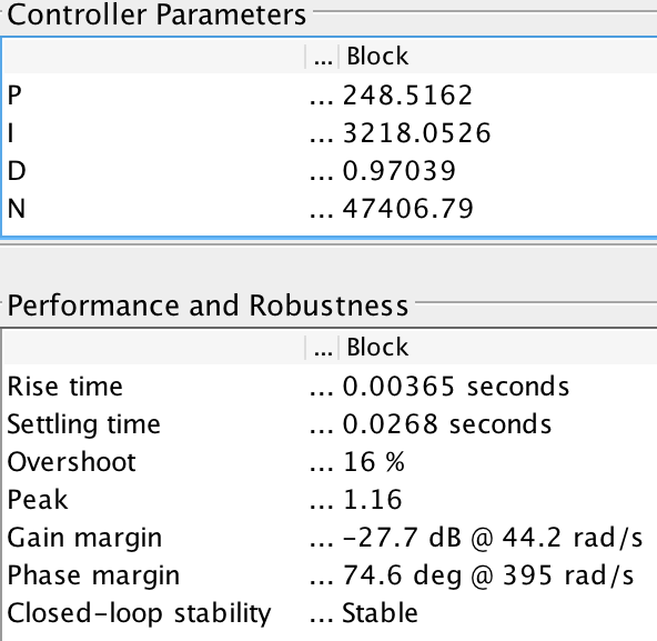
Figure 8:
PID Tuned Parameters and System Performance for Joint A

Figure 9:
Step Response and Bode Plot of Reference Tracking for Joint of B

Figure 10:
PID Tuned Parameters and System Performance for Joint B
Results
Our control goal was to have the robotic arm follow the desired path as closely as possible To test the performance of our closed-loop system, we generated x and y vectors simulating a desired path. Using our derived kinematic equations, we solved for qA and qB (as shown in the Plant section). The resulting qA and qB are the inputs to our closed-loop system i.e. we input a desired qA and qB, and the output is the actual qA and qB of the robotic arm using the controller.
Straight Line Path Experiment
Figure 10 shows the results from having the end-effector follow a straight line. We desired x to go from 0 to .0635 m, and y to remain constant at .0571 m.

Figure 10:
Straight Line Path: Desired and Actual qA and qB from the Closed-Loop System
Sinusoidal Path Experiment
Figure 11 shows the results from our second experiment where the path along x remained the same, but the y path was sinusoidal, with an oscillation of .0063 m and an offset of .0571 m.
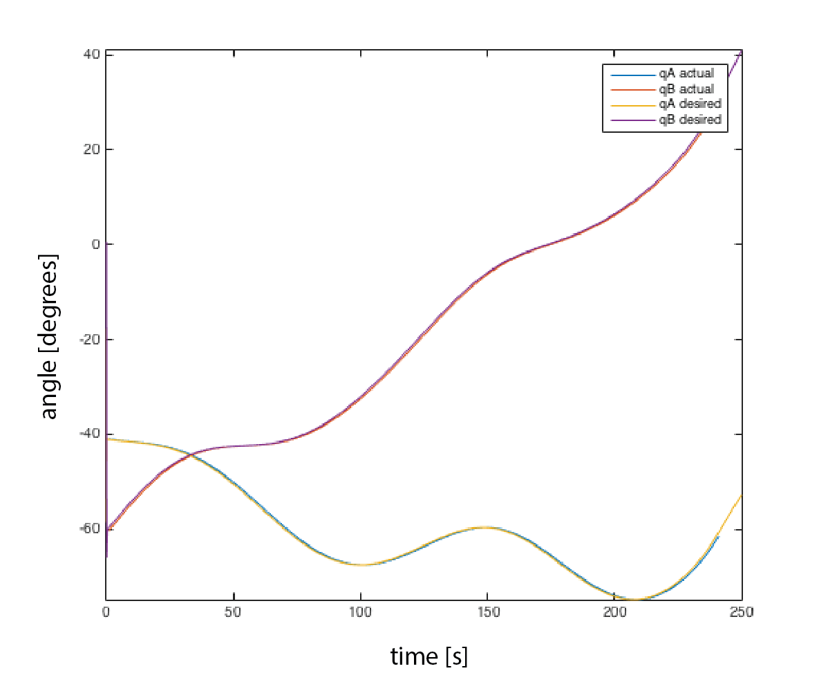
Figure 11:
Sinusoidal Path: Desired and Actual qA and qB from the Closed-Loop System
For both of our planned paths, the system output for qA and qB is very close to the desired qA and qB values. Zooming in on the plots, we see that the steady state error of the system is very small (Figure 12). Our output qA is only slightly larger than the desired qA. The actual qB is slightly smaller than our desired qB.

Figure 12:
Zoomed in plots to highlight steady-state error in straight line experiment and sinusoidal experiment
Unfortunately, the results are not completely good. For both of our experiments, the output values for qA and qB shoot up at time t = 0. Figure 13 shows the same plot from Figure 12 but zoomed in on the zero-crossing.
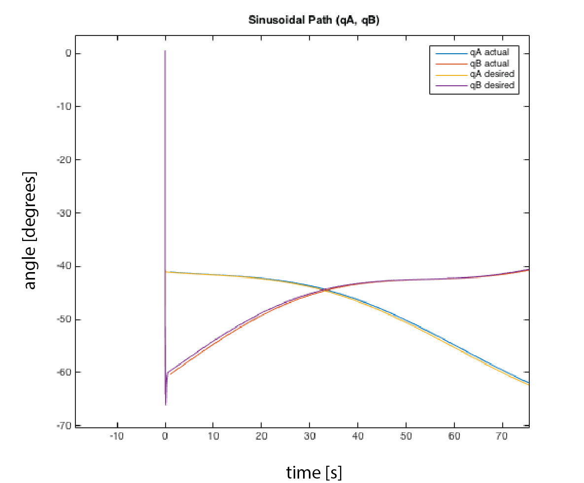
Figure 13:
Zoomed in plot on the zero-crossing (t=0) to highlight unexpected behavior for qA and qB
When we generated the original qA and qB values, we did not encountered this anomaly. However, when simulating the output, Simulink gives the following warning: "The simulation has ignored searching for zero crossing events at time 1.0000248438658845 for (1) zero crossing signals. These signals are being ignored either because their values are smaller than the zero crossing tolerance, or because they caused multiple consecutive zero crossings. This indicates your system is in Zeno, or has strong chattering." To the best of our knowledge, this warning is occurring because of x transitioning from 0 to a positive value. Simulink has a hard time processing this transition, and as such produces the erratic output for qA and qB. Unfortunately, this error is not completely benign. Figure 14 shows the outputs for the x and y paths in both cases. Near time t = 0, the arm behaves extremely erratical and the path is incomprehensible. After the strange initial values, however, the output x,y paths resemble the desired paths almost exactly (Figures 2 and 3 showed the original desired paths).
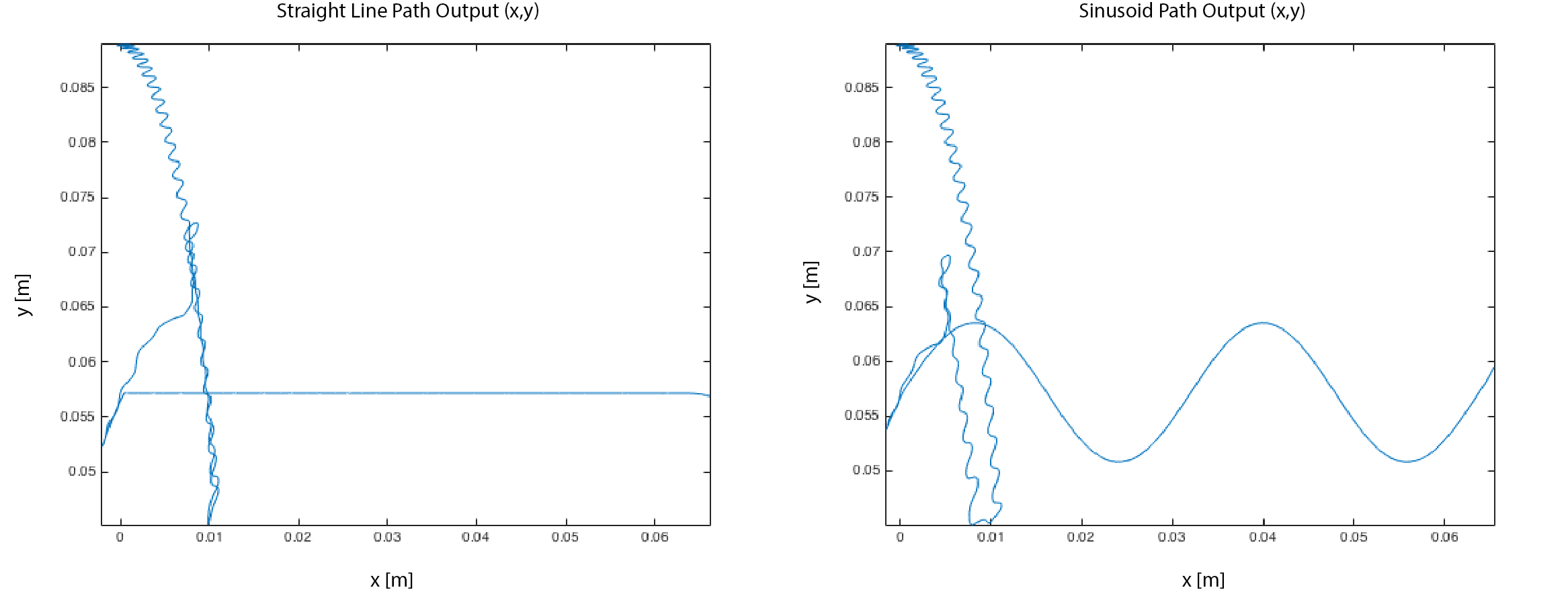
Figure 14:
X and Y Output from the Closed-Loop System
Conclusions
Overall, we are satisfied with the performance of our system. We achieved our main goal of good reference input tracking; the arm's motion is almost exactly what the surgeon desires it to be. The exception to this is, of course, the zero crossing behavior depicted in our Simulink output. We are not sure if this behavior results from a fault in our system or from a limitation of Simulink we overlooked when designing our system. Nevertheless, future work would involve delving deeper into how our system behaves in corner cases like this, and optimizing accordingly. It would also be ideal if instead of two separate PID controllers (one for each joint), our model implemented a 2-input PID controller. This would reflect more the physical reality where the movement of one joint affects movement of the other.
Perhaps the biggest flaw in our model and controller design has been the disregard we've given to important sources of error. To simplify the dynamics, we assumed frictionless arm joints and no damping. Moreover, we have neglected outside environmental disturbances, such as the force of the patient's skin acting against the motion of the arm. Such error would be the chief focus of future work, since it is important for accurate performance. We have also failed to take into account any disturbances resulting from sensor noise. This sensor noise may come from either the actuator itself or the gyroscope used to measure the motion and position of the actuator. Unfortunately, the errors for such devices are incredibly complex and nonlinear. No model we have studied in class can be applied to this error, and as such the benefits of introducing it to our system are questionable. We look forward to learning more about how such errors influence not just our system, but control systems in general, as we continue to advance our knowledge in this field.
Acknowledgments
Caffeine
Files
- Motiongenesis code to derive dynamics equations using Lagrange's method [Attach:MG-code.zip]
- Matlab code for path planning (kinematics) and for interfacing with the Simulink model [Attach:inverseDynamics.zip]
- Simulink model of the open-loop system [Attach:openLoopModel.zip]
- Simulink model of the closed-Loop System [Attach:closedLoopModel.zip]
- User-defined functions for the open-loop and closed-loop Simulink diagrams [Attach:definedFunctions.zip]
References
1.Padoy, Nicolas; Hager, G.D. "Human-Machine Collaborative surgery using learned models", Robotics and Automation (ICRA), 2011 IEEE International Conference on, On page(s): 5285 - 5292
2. http://well.blogs.nytimes.com/2013/02/25/questions-about-a-robotic-surgery/