<<<<<<<

Magnetic Landing Mechanism for First Stage of a Rocket

Ashton Meginnis and Anne-Claire Le Bihan

Abstract

We examine the possibility of landing the first stage of an orbital rocket using a novel method. Magnetic dipoles are proposed as a method of slowing the descent of the rocket. The rocket will be modeled as a magnetic dipole, generated by running a current through the shell. On the ground we have a series of electromagnets generating a strong magnetic field with opposite polarity of the rocket, causing it to slow in its descent. We wish to have a system with near zero overshoot, since overshoot could be catastrophic to the integrity of the rocket and landing pad facility. Our advanced feature is a nonlinear controller due to the nonlinear magnetic force, and an advanced control feature, since we will be using a feed forward control loop.

Introduction

[Due 3/2:] We wish to reuse the first stage of a rocket after it has launched a satellite into orbit. We propose a novel method for the first stage to land. By installing a magnetic dipole in the rocket, we will manipulate the strength of a magnet on the ground to counteract the downward momentum of the rocket as it approaches the landing pad. A proposed method of creating such a dipole on the rocket is to have embedded wires within the shell of the rocket to create a solenoid, and have a battery provide power to the circuit, this creating a magnetic field in the desired direction. We consider atmospheric drag on the rocket and take into account acceleration due to gravity. The magnetic dipole will be activated when the rocket reaches an altitude of 10 km, and we wish the final altitude of the rocket to be 10 meters, at which point we slowly lower the strength of the magnetic field to control the landing of the rocket.

During the descent process, we wish to slow the rocket to near zero velocity at 1 km, so that we can control the remaining descent in a manner that does not harm the rocket or landing pad. The final altitude is 10 meters, so that a platform can be raised to meet the rocket and guide it down to its final resting place. In the project, we are only considering the first stage of this process, in which we lower the rocket from 10 km to 1 km and have it resting there. The following stages are an easy extension of this, as we may now simply lower the magnetic field to slowly descend the remaining distance.

Plant Model

• Description of the landing and of the part of this landing we chose to focus

In order to design a trajectory in which the rocket's stage never hits the ground even when the initial velocity (at z=10 km) is very large, we chose to design our desired trajectory to be a five stage trajectory. The first stage will very strongly and quickly decrease the velocity and the rocket will be stabilized at 1km: at this stage, the rise time and settling time are really unimportant, as long as the overshoot is less than 500m (50%). During the second stage, the altitude of the rocket is held fixed, by keeping the resulting magnetic field in the z perpendicular direction constant and the rocket is moving in the x and y directions, which corresponds to a movement in the North, East, West and South directions, this motion can be from thrusters on the rocket and is outside of the scope of this analysis. The third stage will decrease the altitude of the rocket until it reaches 100m and stabilized it at 100m, the overshoot would have to be less than 50m and again we do not care about the rise time and settle time. Then the fourth stage would manipulate the position of the rocket, so that it willdirectly above the landing pad. The fifth stage will very gently decrease the altitude of the rocket until 10m where it could be grabbed by an elevated platform to lower the rocket the remaining distance. This stage allows minimal overshoot of two meters.

For the purpose of generating this model, we assume that we can create magnetic fields of very high strength, and can direct the field lines in any way we wish. We assume the placement of many of the these giant magnets such that our rocket is descending in a uniform magnetic field generated by the sum of the individual magnets. We assume that the velocity of the rocket is in only the z direction, and the force from the magnets is also in the z direction. This enables us to consider only one dimension in our analysis. Once the rocket has arrived at the desired altitude (either 1 km or 100 m) we can manipulate the strength of individual magnets on the surface of the Earth to guide the rocket to the desired North, East, South, West location - while keeping the altitude fixed - before we continue the descent. As the rocket altitude would be less than 1km during these stages, the rotation of the earth isn't taken into account and we also assume that the magnetic force is far greater than the wind forces which can be neglected. The difficult part of this system would be to slow down the rocket before it hits the ground.

For this reason, we ignore the second and fourth portions of the descent. The third portion, which deals with the descent from 1 km to 100 meters, is a simplification of the first stage, as is the fifth and final portion of the descent. Therefore it suffices to model only the first stage of the reentry and descent, extrapolating to the other stages is simply a matter of changing the constants for the initial conditions and final conditions in the MATLAB code. As mentioned before we model the system of giant magnets as one magnet producing a uniform magnetic field in the region around the rocket. For the first stage, we will analyze a range of initial velocities, which could correspond to different missions. For example a rocket carrying a satellite to GEO would have a different reentry velocity than would a resupply mission to the ISS.

• Equation of motion

We assume the horizontal wind forces are negligible. The forces that apply to the rocket are gravity, magnetic force coming from the magnets and drag opposing the direction of motion.

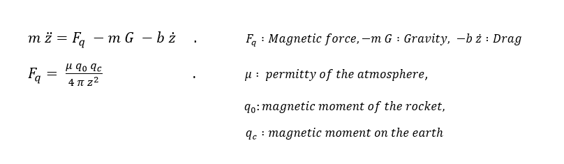
• Parametrizing this system

The mass of a stage of a rocket is approximately 10 tons. As we are adding a parachute to the rocket's stage, the drag is 1,000 kg s/m . G=9.8m/s^2 . We turn on the magnetic field and the initial height Z0 = 10 km. The desired final altitude is Zdes = 1 km. We take a range of initial velocities from 50 m/s to 1,000 m/s depending on the mission in question.

• Modeling of the Fq

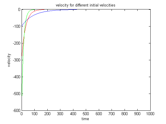
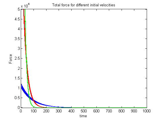
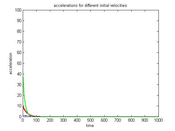
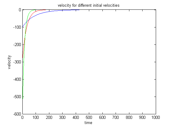
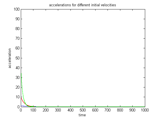
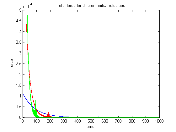
The desired trajectory is a decreasing exponential, which takes the form: v^2 / ( z - Zdes ). And then we calculate F q with the equation of motion. We then simulated this system with MATLAB, using arrays for z, v, a, F q and F tot . We then assume that the measured z at time i was equal to z at time i-1 and that the measured velocity v at time i was equal to v at time (i-1). We chose 3 values of V0 to conduct the simulation and see whether with these assumptions, the system would be able to stabilize the rocket at 1 km without having a too big overshoot. V01= -100 m/s and corresponds to the blue curves, V02= -300 m/s and corresponds to the red curves and V01= -600 m/s and corresponds to the green curves.

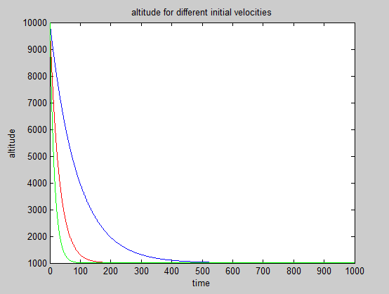
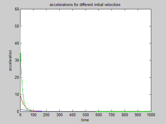
We see that for a normal range of initial velocity, the system is able to stabilize the rocket at 1 km. That is why we set

As A is very well know and I can be perfectly set, q ‘_des_' is exactly equal to q.

Control Design

[Due 3/7:] Give your control design approach.

• First, describe the control approach in words.

From the previous section, we have seen that in the idealized system we described it is possible to control the descent of a rocket using high power magnetic fields. However, in a real system we would not have perfect measurements on the velocity and position of the rocket. So now we are taking into account the possibility for random noise in our measurements, influencing the controller.

The control approach we used was to find an expression for the desired force on the rocket, in order to counter act the downward momentum which exists due to the vehicle reentering the atmosphere. To do this, we model the force as proportional to 1/z^2, we take measurements at each time step of the altitude and velocity. These measurements are used to calculate the desired descent acceleration and force required to slow the rocket to the near zero velocity at the desired altitude.

• Second, give an appropriate mathematical description of your controller.

Our controller in not the standard controller we have discussed in class. It is a feed forward mechanism that relies on a priori knowledge of the desired descent acceleration. The desired acceleration is given by the expression a = v^2/z, where v is the current velocity and z is the current altitude, from this expression we arrive at the total force desired on the rocket F = ma. This force, however takes into account all forces on the rocket, gravity, drag and our magnetic force. From here, finding the magnetic force required is simply, simply subtract the gravity and drag forces. Note however that since gravity points downward and drag is opposite the direction of motion, these terms will appear as positive in the equation. This is the design of our controller.

If we were to physically make this system, once we had the required force from the magnet, we would translate that into a required magnetic moment to be generated from the magnets on the surface of the Earth. Then we would supply the appropriate voltage to drive a current through our electric magnets. This would create the desired magnetic field to slow the descent of our rocket.

• Third, show a detailed block diagram of the closed-loop system, with signals and blocks clearly labeled.

The block diagram is shown above.

• Fourth, explain the derivation of your controller parameters and (if appropriate) the evolution of your controller through the design process. Include information as inline equations, as inline images, or in an attached file.

We began with trying to find a transfer function for our force, which has a 1/z^2 dependence, but found that this was quite difficult to do due to nonlinear phenomena. So instead we took a new approach by modeling the acceleration as a ratio between velocity squared and position. This enabled us to find an expression for the force without having to take the Laplace transform explicitly. With the addition of noise, however, we noticed that our rocket would stop at altitudes that were much greater than the desired altitude, so we added a term to the force this term is proportional to altitude divided by the step time squared.

Expected length: Approximately 1-2 "pages" if this were on 8.5" x 11" paper.

Results

[Due 3/11:] Provide the results of simulations or experiments that clearly show the closed-loop system behavior. Clearly describe the input and output signals.

Preliminary results were listed in the previous sections and our rocket performed nominally. To make the system more interesting we added noise is a variety of manners. In a real situation, no measurement on the velocity or position of the rocket would be perfect and that would subject our system to some errors, which we would have to account for.

In each situation we tested several initial velocities on the system, with each case starting at an altitude of 10 km. Below are some plots of our results.

For this first case, we added error on the measured altitude proportional to the current altitude. The error ranged from plus or minus 10% of the true position.

We notice that even with proportional noise on the parameters the magnetic force is sufficient to slow the rocket within reasonable time. However, upon further consideration we realized that proportional noise is not practical, if we have a rocket at 10 km and have up to 10% error, we have a system that would never be accepted due to high risk involving the error.

The second case of error we analyzed was a linear error, adding some error term to the position plus or minus 20 meters. Below are the results from this case.

Notice how we get some fluctuations in the force, these are due to the error when the true altitude gets near the desired location. The error causes the force to be slightly greater than or slightly less than the desired quantity. However, the response of the system is still nominal and we do not see great overshoot of the desired altitude.

Conclusions

[Due 3/11:] Describe the overall results of your experiment/simulation. Is the system response satisfactory in the context of the application? What would you do in future work if you had more time to work on this? Expected length: 1 paragraph.

Our rocket landing mechanism performed nominally. We saw no overshoot, which was the strictest design requirement. The rise time varied depending on the parameters entered and which method for error we decided to include. This, however, is not an issue; as we stated in the introduction that we are not concerned with rise time as long as the rocket comes down safely. Looking at the required force to be exerted on the rocket, we noticed that the magnetic field would have to be incredibly strong and thus take astronomical amounts of power. So we conclude that this landing mechanism is not the optimal way to return an orbital rocket to the surface of the Earth safely. If we had more time to work on this, we would relax some of the assumptions that we made to make the system more realistic. We would model the force from 4 magnets and have the rocket descend in the middle of them, this would enable us to take into account more than one direction of motion. We could also go deeper into the nonlinear analysis of the system and come up with a better controller for the nonlinear behavior of magnetic force.

While this method may not be optimal for landing a high velocity, expensive rocket; it has been tested to work for wireless bungee jumps. Last year, a team in France constructed a set of four powerful magnets to safely stop a man jumping off a building before he hit the ground. The test worked, here is an image of one of their first tests in which they tested the system with a magnetic ball.

You can find the entire video here: https://www.youtube.com/watch?v=8M6M1ZDo8N8

Files

Code and Simulink models should be linked here. You can upload these using the Attach command.

• Modelization of F _q : MATLAB code

As we want the trajectory to have a rough shape of a decreasing exponential, we want roughly the acceleration to be roughly equal to : v ² / ( z - z _des ). And then we calculate F _q with the equation of motion. We then simulated this system with MATLAB, using arrays for z, v, a, F _q and F _tot . We then assume that z _measured at time i was equal to z at time i-1 and that v _measured at time i was equal to v at time i-1. We chose 3 values of V0 to conduct the simulation and see whether with these assumptions, the system would be able to stabilize the rocket at 1 km without having a too big overshoot. V01= -100 m. s ‘^-1^' and corresponds to the blue curves, V02= -300 m. s ‘^-1^' and corresponds to the red curves and V01= -600 m. s ‘^-1^' and corresponds to the green curves.

Attach:codesimulation1.pdf

• File 2 attached and described here
• File 3 attached and described here

References

List the referenced literature, websites, etc. here.

---