Airplane Landing Control

Project team member(s): Caroline Fong and Sharon Tseng

Abstract:

This system models the final leg of an airplane descent to a destination -- more specifically, the final leg of descent when the airplane has a relatively straight path down to its landing area. With various forces acting on the plane (gravitational, air resistance, lift, thrust) at a given angle, the pilot uses GPS to verify that the plane maintains it's path as it descends and corrects as needed using feedback controls. Below, we find a PD controller to control the thrust force based on the specified horizontal, x-direction motion. We chose this project because we had previous experience working on GPS feedback on cars and the goal is to allow the airplane to land safely in a reasonable amount of time without too much veering off course.

Advanced Feature: The advanced feature of our project is a Simulink model of the nonlinear system.

Introduction:

An airplane's descent is a complicated, yet important stage of the flight. Our system refers to the final leg when the airplane has a relatively straight path down to its landing area. In this scenario, there are multiple forces acting on the plane (lift, thrust, weight and drag) at various angles. The weight is the force due to gravity on the airplane which is opposed by the lift, the air flowing over the wing. Thrust is created by the propellor and opposes drag, air resistance on the airplane. To land, the thrust must be less than the drag and the lift must be less than the weight.

To make sure the plane lands on the runway, a pilot uses GPS to verify that it is still on the right path as it is descending and corrects as needed using feedback controls. Since GPS is usually accurate to about a meter, it is important to make sure that the plane responds accurately. In addition, a plane can end up burning a lot of fuel and wasting precious time in its narrow window for landing if it ends up having to correct its path too frequently because of a poor feedback control system. We chose this project because one of us worked on GPS accuracy and feedback over the summer for self-driving cars and thought it would be interesting to see how GPS feedback would operate on a much larger vehicle with different forces acting on it (an airplane).

Plant Model

Our model will look at a GPS controlled airplane's descent. We will focus on the horizontal motion (in the x-direction) of the plane, assuming that the change in horizontal motion is much greater than the change in vertical motion. The reference is the desired path for the airplane to take and is controlled using a GPS, which tells the plane where to go. We will assume that the plane's angle is a constant 5 degrees throughout the descent. We will also model the drag and lift force as viscous damping.

Based off of our model, we found that the time domain equation of the forces in the horizontal, x-direction. We assumed that F_drag went as b*x'(t).

The two parameters for our model are the mass (m) of the airplane and the damping (b) force from drag. We will also assume, for the time being, that the angle of descent is 5 degrees, which allows us to linearize the equation of motion. The mass of our airplane is the lower range for a 747's maximum takeoff weight, 333,400kg. Even though we are modeling the descent of the plane, we are assuming that the 747 starts out greater than this takeoff weight and will burn fuel during the flight. The drag force on the airplane we estimated using the drag force equation: D = Cd x p x V^2 x A / 2. The drag coefficient for a Boeing 747 is 0.031. A Boeing 747 has a cruising altitude of about 10,000 m so our model looks at the plane right when it starts its final descent, at around 3,000 m. At this altitude, the density of the air is 0.9093 kg/m^3. The velocity is from the approach speed of a Boeing 747 which is about 150 knots or 77.167 mps. For the area, we looked at the drag on the airplane's wings. Each Boeing 747 has a wing area of 541.2 m^2 so our total area is 1082.4 m^2. So: D = 0.031*0.9093*(77.167)^2*1082.4/2 = 90,926.600N.

Our open loop simulation shows that there is no settling time for the system. That suggests that the airplane will never reach it's desired path, which would be problematic during the crucial moments of an airplane's descent.

Control Design

To control our system, we initially decided to use a PID controller over a PD controller because the system is very sensitive to the final value. The plane must land on the runway so having too great of a steady state error would have fairly disastrous effects during landing. This is mitigated by the Ki term, which eliminates bias offset. To start, we implemented a PD controller and then planned to use those values to design a PID controller. For our PD controller, we started by setting constraints that the settling time had to be less than 30 seconds and the overshoot had to be less than 5% . We then calculated that Kd = 11,316.1 and Kp = 0.05. After testing it in MATLAB using a step response, we modified the values to a final Kd value of 1500 and Kp value of 2500 because our initial values had too large of a Kd value and too small of a Kp value. In addition , we wanted to ensure that our settling time was not more than a couple of minutes long. We then plotted the step response on MATLAB to see how the airplane reacts given a constant thrust after no thrust. That gave us the following graph and parameters:

Equations to find PD K values.

From there, we tried to implement a PID controller but found that adding the integral term increased the overshoot and settling time drastically while only decreasing the settling value marginally. For instance, with Ki = 10, the system had the following response:

Step response with a PID controller.

Rise time: 55.3803 Settling time: 533.4081 Settling min: 0.9078 Settling max: 1.0972

Peak time: 162.3509

The settling time more than doubled and the system now has an overshoot of 9.7% when it didn't have an overshoot beforehand. The new PID controller now has a greater range of settling values, that better centers around 1 but also has twice the margin of error. Thus, we decided that a PD controller would be sufficient. Our final PD controller is:

Advanced Feature: For our advanced feature, we chose to implement a Simulink model of the nonlinear system. This mainly modified the m term in front of the s^2 term into m/cos(theta) where we specified the theta was 5 degrees. Our two different systems are shown below:

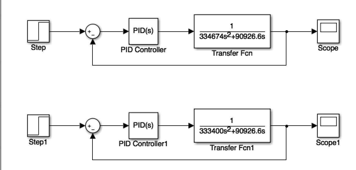
The top system is the nonlinear system while the bottom system shows the linear version.

The linearized and nonlinearized versions had very similar responses in Simulink. For instance, both showed the same transient response with steady state errors that are not discernible in the Simulink models. Both have about the same rise and settling times as well. This shows that the linearized version of the system approximates the real system (nonlinearized), extremely well so our model would approximate the real system relatively well, based on the original equations of motions we derived.

This is the Simulink model response to the linear system.

This is the Simulink model response to the nonlinear system where theta is 5 degrees.

We also decided to test the performance of our PID if we assumed that the descent angle, theta, was 20 degrees. As pictured below, the time response is still quite similar to our linearized solution, once again showing that the linear system is a good approximation for the nonlinear system. Thus, throughout the descent, where the maximum descent angle would be around 20 degrees, we can use the linearized system. This is most likely due to the fact that the mass of the airplane is so large that there is a greater tolerance on the "small angle approximation."

This is the Simulink model response to the nonlinear system where theta is 20 degrees.

Results

We control the airplane path using a PD controller (D = 1500s + 2500) to have a rise time of a few minutes max, a very small steady state error and not too large of an overshoot or undershoot fluctuation. We chose these parameters specifically because of the need for accuracy in landing a plane and also because all of the forces on the plane are so large that fluctuations would be too unwieldy to play out in real life. The response to a step input is shown again below.

The input to this system is the thrust on the plane and the output is the actual x position of the plane. When the system (with PD controller) is applied a constant thrust from no thrust, as shown by the step response, there is no overshoot or undershoot which is easier for the plane to handle. In addition, it has a rise time of of 1.5 minutes, a perfectly acceptable amount of time in the ten or more minutes of final descent for a plane. The settling time has a maximum of almost exactly the expected value and at most deviates by 10%, or a couple dozen feet from the target position on the runway.

Modeling our system using Simulink revealed that the linear and nonlinear systems had almost exactly the same transient values. This gives us increased confidence that the control design we propose will work as we predicted in our simplified linear system.

Conclusions

The simulation was fairly effective in that it met all of our initial target requirements. The only requirement it may not pass would be the steady state error since even small percentages of steady state error translate to many feet in real life because of the scale of our project. The next stage of the simulation would be to examine how the angle of descent affects the system. For this system, to model a single input single output system, we set the descent angle, theta, to be constant. However, we could model theta as a disturbance and see how the system responds to that. Though we created equations to describe both horizontal and vertical movement of the plane in descent, we chose to only examine the x-position of the plane. A more elaborate simulation could examine both components to determine if the plane lands in both the desired horizontal and vertical lengths.

Acknowledgments

Thank you to Professor Allison Okamura and Adam Leeper for a wonderful quarter learning about feedback control. Also, thank you to Tania and Kirsten who were very helpful in the implementation of this model.

Files

• To view our MATLAB code regarding the open and closed loop control systems: Attach:Fong_Tseng_MATLABcode
• To view the Simulink analysis for the nonlinearized systems: Attach:Fong_Tseng_Simulink

References

http://www.pilotfriend.com/training/flight_training/aero/forces.htm

---