Z-Axis Stabilization on a Descending Rocket via Actuated Fins

Project team members: Andrew Nguyen and Chris Kimes

Abstract

Hobbyist rocket launch and recovery can be an unpredictable process with many variable factors that may affect the launch trajectory, descent path, and physical integrity of the rocket. The process includes many areas where a control law could add stability and account for variability to provide some level of predictability in the launch. For our project, we will be stabilizing the z-axis spin of descending rocket after its launch using actuated fins to provide a lift force against it's angular motion. Our goal is to take a rocket-parachute system with z-axis spin and apply an angle of attack with the fins to bring its angular velocity to zero.

Advanced features we're including in our system will be a time delay from the sensor in the feedback path. The sensor will introduce a delay through the averaging of angular velocity measurements to remove spikes in the measurements and noisy values. Our goal for control design will be to create a controller that will account for time delay and its tendencies to add instability to the system.

Introduction

We wanted to find out if we could control z-axis spin in a rocket during its descent through a unique pair of actuated fins that would pop out sometime during the launch or descent. The purpose of controlling the z-axis is to solve part of the controls problem that comes along with attempting to land the separate stages of a rocket or any other object. We figured that tackling the z-axis spin was a suitable controls problem for our final project and would be a solid first step towards a stable land. However in this system, the fins will be on the second stage of the rocket that carries the avionics package and payload for the rocket. The problem comes from a Stanford Student Space Initiative rockets project that needs the controls math for the z-axis stabilization for their descent. Realistic parameter values such as the moment of inertia from the fins, the area and offset of the fins will be provided by the SSI rockets team for us to work with.

Plant Model

To control our z-axis rotation, we control the angle of two control fins attached to the side of a rocket during its descent. The fins exert a lift force L, which depends upon the fin angle, z-axis rotational velocity, and physical constants. We have derived the following linearized equation of motion:

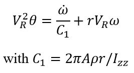
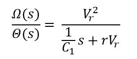
where θ is the fin angle from the vertical, ω is the rocket's z-axis rotational velocity, VR is the rocket's descent velocity, r is the radius from the rocket's central axis to the center of the rectangular fin, A is the fin area, ρ is the density of air, and Izz is the rocket's moment of inertia about the z-axis. See the attached document for derivation of this equation. This time-domain equation of motion yields the following S-domain transfer function:

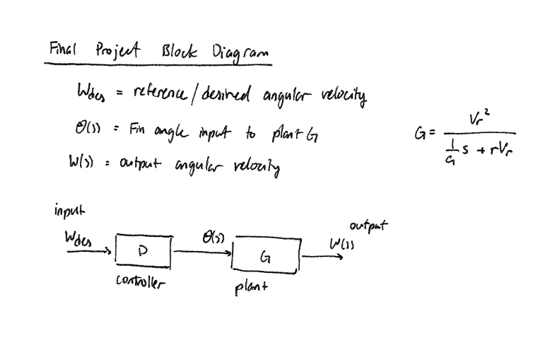
Block diagram of model:

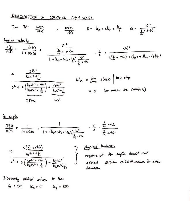
Derivation of model as shown:

Since this project will be working in collaboration with one of the rockets team in SSI, we will use the parameters of their physical system in our model of the system. Based on Solidworks data on a model of the fins and rocket, we have the moment of inertia for the fins to be 0.006916857378 kg*m², the fin area to be 103.226 cm² and the radius from the rocket's centerline z-axis to be 5.11cm. In our linear approximation of the model, we define V_r to be a constant during the descent, which SSI has defined our landing velocity to be 5.273 m/s.

First Pass Simulation and Analysis

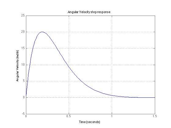
This is a simulation of the step response of the plant in open loop configuration. The input is a step response scaled to represent an input fin angle of ~5 degrees, while the output of the system is the angular velocity of the rocket. The problem with this simulation is that steady-state values do not go to zero like we desire, rather they reach some value that does not match the goal of the system. The next step is to incorporate a controller that reads in the error in measured angular velocity and desired angular velocity and convert that to an appropriate fin angle.

Control Design

SSI has asked us to implement a simple PID controller to control fin angle. This controller will have a transfer function given by:

With this PID control law, the system output becomes type one with respect to a disturbance. This means that a PID controller will consistently drive the rocket's angular velocity to zero in the presence of any naturally occurring disturbance. While this means any PID parameters we pick will still drive the system's response to zero, we had to tune our controller to account for physical limitations for both ourselves and SSI's hardware. For example, to comply with small angle approximations in our initial linearization, we want to limit our fin angle to no more than 15 degrees, or 0.2618 radians. On the other hand, we realistically expect our system to respond well to angular velocities of up to ~25 radians/second, which corresponds to 240 rpm.

The following block diagram shows the updated, block diagram after adding our PID controller and closing the feedback loop. We assume that our system is subject to a disturbance V(s). This disturbance term can account for small changes in air density, wind velocity, or other disturbances that would affect the angular velocity.

Here is the derivation of our PID control parameters:

Using this initial model of our control system, we found the step response for both theta and omega for a disturbance in theta. % % We eventually decided to change how we modeled our disturbance to better reflect the physical rocket system and how we expect it to perform, more on that below.

Results

After initially choosing to respond to disturbances in theta as described above, we decided that it would be more physically realistic to respond to an initial angular velocity and then drive it to zero. After the launch phase, we feel that the most likely use of our control system would be stabilizing an initial spin once the control system is activated during the descent. This new mode of operation is described by this block diagram:

To model this, we could either perform a change of variables and model the resulting non-linear system, or use Simulink to model a custom step response. Since Simulink is easy to use (and we'd have to use it anyways for the nonlinear change-of-variables approach), we'll use it to create a custom step response. We will allow our system to reach steady-state at omega = 10 rad/s, then drop the step off to zero, which occurs at 5 seconds. Rather than re-derive constants to be used in the control law, we utilized Simulink's PID tuning functionality to find constants that would meet our performance requirements. We found:

Kp = 0.0362, Ki =0.00703 and Kd = -0.0277

Note that we do not care about the response for rising to 10 rad/s, only that it equilibrates. This is important for our assumptions, particularly the small angle approximation. We have chosen a relatively tight small-angle threshold of 0.26 radians (15 degrees). This means that our system and PID controller should not create an angle theta with magnitude greater than 0.26, otherwise the our system will no longer adhere to our assumptions and uncertainty will result.

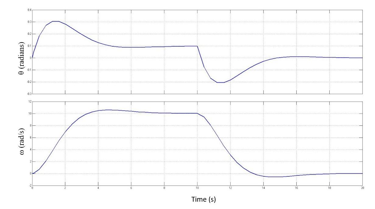
This image is a scope output from Simulink; the top plot is theta vs time, the bottom plot is the response omega vs time. note that the magnitude of theta exceeds 0.26 radians while rising initially, but for the part of the plot that matters, when the system drives omega to zero, theta does not exceed this value.

We also chose to model the time delay of the system. While we do not have hardware specs from SSI for modeling this time delay, we assume that their relatively inexpensive hardware will have some appreciable delay in sensing and calculating the angular output, so we'll assume a worst-case time delay of 0.1s. We modeled this using both a (2,2) Pade approximation and using Simulink's non-linear simulation, and the results were very similar, so we've only uploaded the version using Simulink's non-linear time delay.

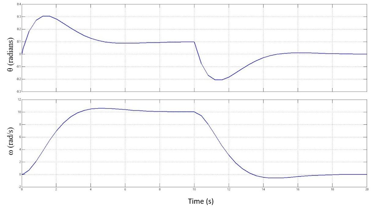
Using the control gains prescribed by Simulink's PID tuning function, we were able to find a quick response to an initial angular velocity while accounting for a generous time delay in the feedback path. Our response stayed within the physical limits of our system while stabilizing the z-axis spin in around six seconds.

Conclusions

Through many iterations of our block diagram, PID constants, and methods to model initial conditions and disturbances, we designed a controller and a reasonably accurate model of our system for which we could predict a stable reduction of angular velocity to 0 rad/s via control of fin angles. Given more time to work on this project, we would have more physical meetings with SSI to refine the parameters of the rocket and make sure that our initial assumptions were correct with their assumptions. It would be more helpful to match up our physical limitations we imposed on the system with their limitations, such as maximum expected controllable angular velocity and maximum fin angle. Since their launch was pushed back, it was not necessary to fulfill their requirements for a launch in order to finish this project for the class. On our side, we would like to refine our controller more and be able to report a range of values for initial angular velocity for which the system is stable. Ultimately, from what we learned from our design process and the dynamics of the system, we are confident that with some sanity checking with SSI, our controller will be able to achieve its primary purpose. After this class, Andrew will continue to work with SSI to see this project through!

Acknowledgments

We'd like to thank SSI Prometheus Team for providing data on our physical system for their rocket. We're super excited to be able to collaborate with the team and hopefully have our control system used on their launches!

Files

Here are the Matlab and Simulink models we used for the majority of our analysis:

Our initial Matlab modeling script, as well as Simulink models used for later iterations are here:

%Attach:NguyenKimesStuff.zip

References

Franklin Powell Emami-Naeini Feedback Control of Dynamic Systems, 7th Edition

---