

Connor Anderson Ben Cohen
Hydrofoil Control In High Performance Sailing
Project team members: Connor Anderson, Ben Cohen
Abstract
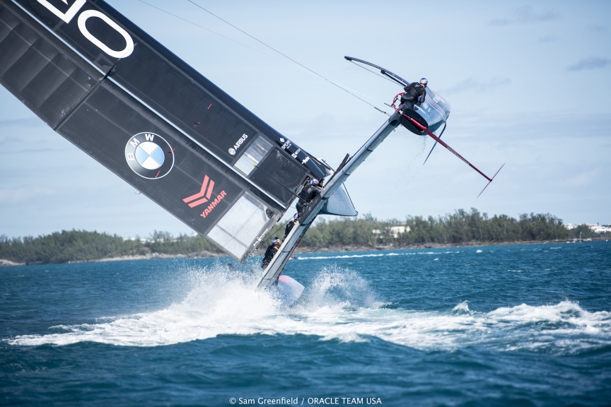
Hydrofoiling sailboat
Our project focuses on the controls necessary to optimally manipulate the hydrofoils on an advanced sailboat. The project is motivated by a general interest in high performance sailing, and a separate but related project. Our goal is to maintain a stable pitch of the hull above the water by controlling the pitch of the rear hydrofoil--the front hydrofoils are assumed to be fixed at the nominal angle of attack which keeps the boat in static equilibrium.
In order to get a usable transfer function, we first solved for the nominal, steady state front and rear angle of attack that would keep the boat level. We then redefined a new angle that was the sum of the variable for the rear angle and the nominal steady state value of the front angle. This allowed us to simplify our function into terms dependent only on the boat's pitch, and a new variable that accounts for the angle of both the front and rear hydrofoils.
After designing a lead-lag compensator, we created a system capable of tracking a step input and disturbance with no error. Our system has a satisfactory overshoot and settling time of 3.5 degrees and 3 seconds, respectively.
Introduction
Advanced sail boats use hydrofoils to increase speed by lifting the hull out of the water to decrease drag, which scales with the square of the boat's velocity, and depends on the viscosity of the fluid surrounding the hull. So, because water is more viscous than air, it is advantageous to have the hull move through the air. Once the hull of the boat is out of the water, the hydrofoils must maintain a constant depth, so that the hull does not become submerged in the water, which can happen if the hydrofoils rise too high (the boat comes crashing down), or too low. Our project will investigate the relationship between the pitch of the hydrofoils and the pitch of the hull itself, and will explore the controls necessary to create an optimal system.
Plant Model
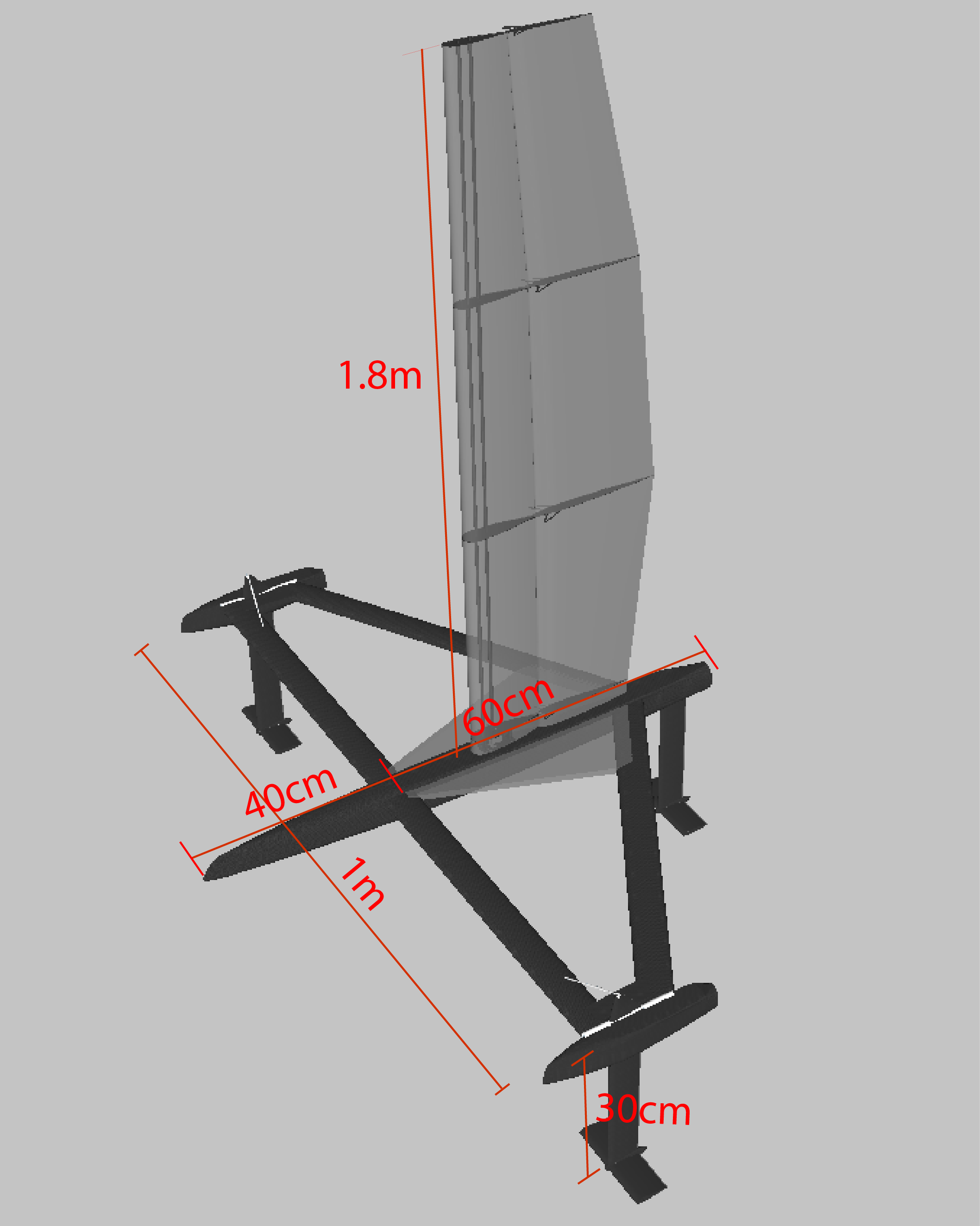
Reference Geometry for Analysis
| Parameter | Value | Description |
|---|---|---|
| V | 4 knots | Constant velocity of boat |
| ρw | 1000kg/m3 | Density of water |
| ρa | 1.23kg/m3 | Density of air |
| Fsail | Variable | Variable driving force from sail |
| A | 0.009 m2 | Planform area of hydrofoil |
| I | 8E-4 kg*m2 | Moment of inertia about CM |
| Cl | variable | Coefficient of lift of hydrofoil |
| Cd | variable | Coefficient of drag of hydrofoil |
| Θ1 | Independent Variable | Angle of first hydrofoil |
| Θ2 | Independent Variable | Angle of second hydrofoil |
| h | variable | Height of boat above water |
| Φ | variable | Pitch angle of boat |
| C1 | 0.1 | Constant linear lift scaling |
| C2 | 2.5E-4 | Constant drag scaling |
| Offset | 0.4 | Offset for cl equation |
| Offset2 | 0.01 | Offset for cd equation |
| Mass | 2kg | Mass of boat |

Analytically Determined Performance of SD7043 Airfoil with 2d Hydrofoil Analysis
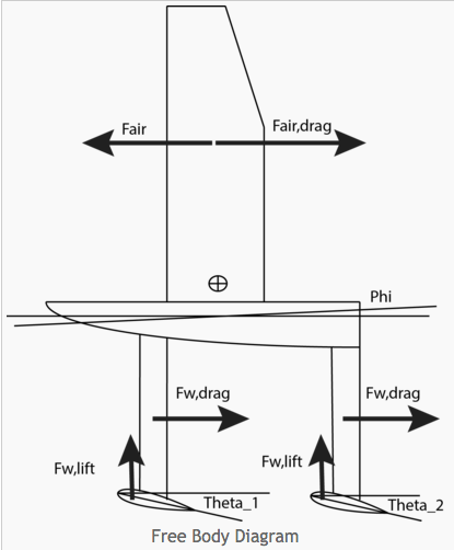
Derivation of Equations of Motion
Our model is a 2D representation of the side of a sailboat. We are not taking into consideration the yaw or roll of the boat, only its pitch, so this representation should be sufficient. We will model the boat as having a drag force from both its submerged components � the hydrofoils � as well as its hull and sail, a driving force from the wind in the sail, and two lift forces from each of the hydrofoils. To simplify the model, we will assume the sail provides a constant force forward, and that the hydrofoils are connected to the hull by components that create such small drag forces that they can be neglected.

Laplace Derivation
Taking the Laplace of the time domain equation � the equation of motion taken about the center of mass, we get

At this point, we do not have the mathematical tools to solve for the transfer function ϕ(s)/θ_2 (s) or ϕ(s)/θ_1 (s), or even ϕ(s)/〖(θ〗_2 (s)-θ_1 (s)). If we take the moment about either hydrofoil, we can eliminate its contribution to torque, but will still have a constant term from the torque contribution of the sail and hull. We also cannot simplify the equation to combine the two hydrofoil pitches into a 〖(θ〗_2 (s)-θ_1 (s)) term, because of their different coefficients.
Because of this, we decided to fix our first hydrofoil at its nominal value, and only rotate the rear hydrofoil. This simplification allows us to model the system as a SISO. Using this simplification, we also are able to remove the constants that appeared in the initial analysis by remapping θ_2 to a new variable, θ_3. This new equation takes the form: θ_3 = θ_2 + θ_2nom or more specifically θ_3 = θ_2 + 1.1639�. The derivation for this nominal value is included for reference in the NominalThetaCalculations.pdf file attached to this webpage.
Using the nominal θ_1 value, and the new mapping of θ_2, we can solve for the transfer function of our system. Solving the equation of motion with these values, we get a simplification of:

At this point, we linearized the above equation to remove the θ_2^2 component because it is much smaller than the other terms. In this way, we can establish our desired equation to relate θ_3 to the left side of the equation.

Taking the Laplace transform of this equation, we arrive at our final system transfer function:

Block Diagram Model
For our block diagram of the open loop system, we model the overall transfer function of the system. This includes the main plant transfer function as well as a gain to convert from radians to degrees (needed for the input of the plant). Additionally, the summation block at the top would be the branch that actually controls the angular position of the hydrofoils, since it remaps θ_3 back to θ_2.

Control Design
Our control approach implements a lead-lag compensator. The lead compensator�derivative control�adds phase to the transfer function's constant phase of -180 degrees to increase the phase margin and dampen the system. The lag compensator�integral control�eliminates the steady state error in the system response, increasing the system type.
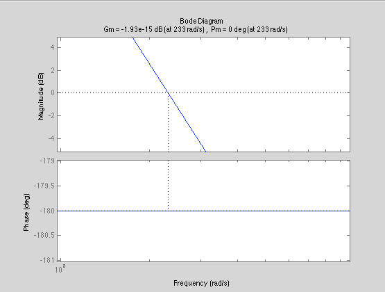
Transfer Function Bode Plot
Our lead-lag compensator adds a poll at the origin and two zeros at 1 rad/s and 20 rad/s, with a gain of 0.25 to achieve a high phase margin and subsequently a smaller overshoot. The format of our compensator is shown below:

This iteration of our controller design resulted in the best disturbance rejection and most ideal damping, giving us our fastest response time. Additionally, we added a fast pole at -10,000 to make it possible to simulate this block in MATLAB. Below is the closed loop block diagram for the system:
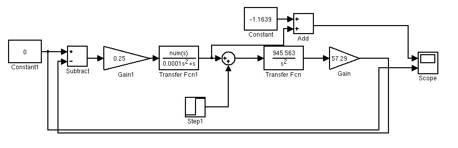
Closed-Loop Block Diagram
Our compensator design started with a damping term (Td) of 20 rad/s which is one decade lower than the original crossover frequency. Then, to maintain the ideal Ti/Td ratio of 20, our integral term was set at 400 rad/s. We then chose a very small gain of 3*10^(-7) to offset the large gain of the bode plot in a way that would yield a large phase margin.
Step Input Tracking
Step Disturbance Rejection
Although this compensator tracked the input well, it exhibited too slow of a response to a disturbance--one of our advanced features--so we decreased our integral term by another decade, and then decreased our derivative term to maintain a Ti/Td ratio of 20. We decided to design for disturbance rejection as well as input tracking because it seemed like a more realistic objective for sailing. As you can see below, our system is type one with respect to disturbance:

With the new Ti and Td, we again plotted the system with a gain of 1, and then manipulated the gain such that the phase margin was around 70 degrees. As shown below, this yielded a better response time, however from the bode plot it was clear that there was still room to increase the gain and as a result, the phase margin.
Step Input Tracking

Step Disturbance Rejection

Bode Plot
For our third and final iteration, we merely increased the gain of our compensator by a factor of 10, to arrive at a phase margin of 84.4 degrees. Our response exhibited satisfactory disturbance rejection and input response, so this became our final design.
Step Input Tracking
Step Disturbance Rejection

Final Design Bode Plot
Results
After establishing our controller design, we were able to simulate the input reference tracking. We also know that our system is Type 1 with respect to disturbance, so we expect 0 error with respect to a step disturbance and constant error for ramp disturbance. We also are nicely able to track a step and ramp input, as well. The following images show how our final controller successfully met these criteria:
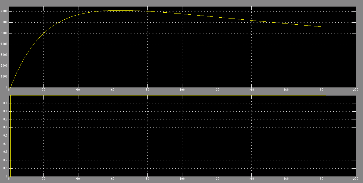
System Response to Ramp Input
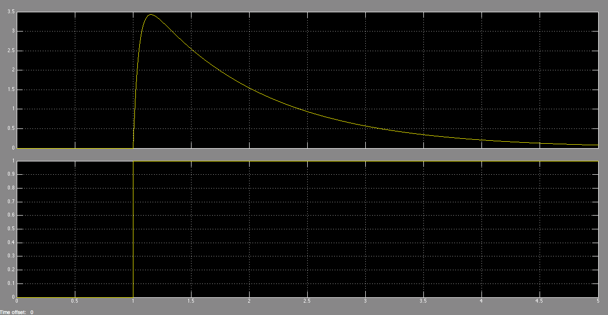
System Response to Step Input

System Response to Ramp Disturbance
System Response to Step Disturbance
We can also look at the output plot for 𝞱1 over time to get an idea of how the hydrofoil is reacting to the input reference. As we can see in the figure below, we jump to around a peak of 12� before returning to the nominal value of -1.16�. This is an optimal range because we stay within the linear region of the hydrofoil, which gives us the most accurate control. However, the response time is much faster than we could likely achieve with any reasonable servo, so in the future, some work will have to be done to factor in the mechanical time constant of the system in order to determine a reasonable amount of time that the system can actually adjust to a given desired input.

Theta2 Response to Step Input
Additional Advanced Applications
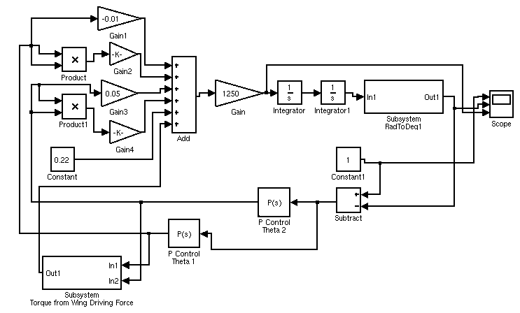
Ideally, we will not just fix the first hydrofoil, but will individually control both to give a faster overall system response. This advanced control approach implements a linear controller in a nonlinear system, to control the angle of attack of each of the two hydrofoils. The complexity of our block diagram is a reflection of our equation of motion, which is second-order in each of the angles of attack:

Our controller for this system is a P controller, whose input is the pitch angle of the entire boat. Given that there are many parameters to calculate to stabilize this system, we would ideally start with calculating a proportional term, and then add complexity to fully stabilize the system and eliminate steady state error. It also may be possible to incorporate the lead-lag compensator from our primary control design on both hydrofoils, although we were not able to implement this due to time constraints. The controller uses two separate gain values to calculate the proper pitch angle for each hydrofoil, which are then sent through the nonlinear system. The complete block diagram for this analysis is shown below:


Conclusions
After many iterations, we settled on a system model and controller that satisfied our design goals of system response to both input and disturbance. The simplifications made to our system model allowed us to get a transfer function we could fully analyze, and so we were able to apply and analytically manipulate a lead-lag compensator to yield a system that is type one with respect to disturbance. This satisfies the requirements for the physical system, as the boat can track a step input for its pitch, and it can reject disturbances--say a gust of wind or a wave--that resemble an impulse or step. With more time, we would focus on controlling both hydrofoils rather than just one, and would seek to more accurately model the non-linear elements of our system.
Acknowledgments
Special thanks to Allison Okamura and Adam Leeper for putting up with so many questions. Thanks to robotics club team members Isabel Gueble, Wyatt Smith, Schuyler Smith, Thomas Teisberg, and Andrey Sushko for helping make this boat a reality.
Files
- File 1: Full Closed Loop Simulink Model
- File 2: Calculations and Code for Adjusting Various Boat Parameters
- File 3: Function to Find Nominal Hydrofoil Angles
- File 4: Script to Find Transfer Functions of System
- File 5: Script to Compare Various Boat Parameters