

Elizabeth Neville Sohrab Godrej

Effect of a Nonlinear Disturbance on Vehicle Cruise Control
Project team member(s): Elizabeth Neville and Sohrab Godrej
Abstract
In this project we examine the cruise control system in a standard passenger vehicle. The technology behind cruise control is increasingly important with the advent of self-driving cars, as these vehicles will need to be able to regulate their speed effectively and autonomously. Specifically, we examine how changing the slope of the road (modeled as a nonlinear disturbance input) affects the cruise control system. We will demonstrate that the effects of this disturbance are minimized through the implementation of a PI controller and the addition of a low pass filter to minimize controller effort over bumpy road surfaces.
Our project's advanced feature will be a Simulink model of the nonlinear system (the governing equation includes an mgsinθ disturbance term where θ is the slope of the road)
Introduction
Cruise control is a convenient feature in many automobiles because it allows the driver to rest his/her foot off the gas pedal along a relatively straight stretch of road while the car control system keeps the velocity constant. Looking to the future, this technology is extremely relevant to the control systems of autonomous vehicles as well, since these systems must have the ability to consistently and effectively regulate vehicle velocity at all times. The governing equation for the car's velocity, v, depends on the mass of the vehicle, m, the gravitational constant g, the air resistance damping term c, the slope of the road theta, and the controls signal (related to the force applied by the engine) u.
v ' + (c/m) v = u - gsinθ
Plant Model
1. Description of Model
The forces acting on the vehicle parallel to the road are the force of gravity (related to the slope of the road, θ), the force of air resistance (related to velocity and the air resistance coefficient c), and the force produced by the engine. The resulting motion m*a (or m*v' in our equation) is given by the sum of all these forces.
2. Equations
Time Domain Equation
v '+ (c/m) v = u - gsinθ
Laplace Domain Open Loop Transfer Functions
With respect to controller input, u�.
V/U = 1/(s+c/m)
With respect to incline angle, θ (linearized about θ = 0; must use Simulink to model nonlinear system)
V/θ = -g/(s+c/m)
3. Open Loop Block Diagram

4. Derivation of Model

5. Parameters
| Parameter | Description | Value |
| v | Velocity of car | Variable |
| u | Controller input | Variable |
| θ | Angle of road incline | Variable |
| m | Mass of car | 1270 kg [1] |
| g | Gravitational constant | 9.8 m/s^2 |
| c | Air resistance damping coefficient | 25.4 kg/s [2] |
[1] Approximate mass of a standard compact car
[2] Paramater for an Audi in 4th gear (found online, source below)
6. Simulation
The plot below shows the response of the open loop plant model to a step input of 60 (corresponding to a desired velocity of 60 mph),as well as a step disturbance input of pi/3 (corresponding to a constant road angle of 60 degrees as the car ascends an incline of constant slope).
Open loop response to a step input of 60 mph, constant road angle of 60 degrees
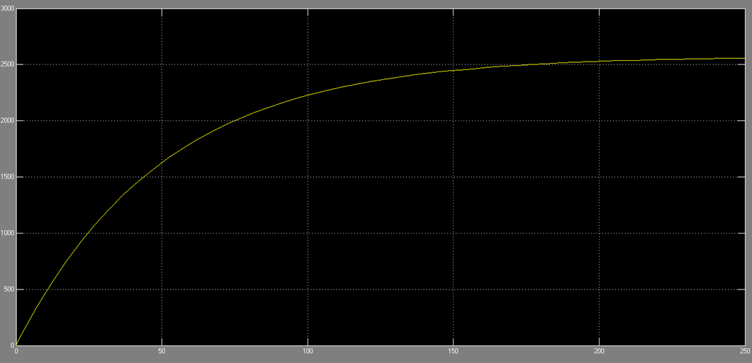
The open loop behavior of the plant is clearly unacceptable as the steady state velocity reached is over 2500 mph, which is nowhere near our target speed of 60 mph (and also physically unrealizable). Additionally, the open loop system takes over 3 minutes to reach this steady state value, an unacceptable settling time in the context of highway driving.
Control Design
1. Control Approach
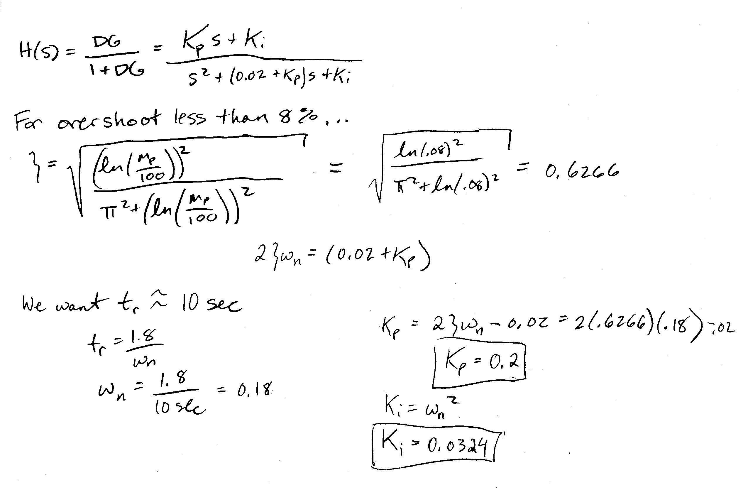
As observed in our open loop simulation, there is a large, finite steady state error in the plant response to a step input. To bring this error down to zero we chose to add an integrator in the form of a PI controller. This brought the system type from Type 0 to Type 1 and brought the steady state error of the response with respect to controller input as well as with respect to disturbance input down to 0. We chose our gains Kp and Ki such that we would achieve a rise time of around 10 seconds (as accelerating from 0 to 60 mph any faster than this could become unpleasant for passengers). We also aimed for a maximum overshoot of no more than 8%, the equivalent of about 5 mph when the target value is 60 mph (this is so that in the process of getting to 60 mph, the vehicle does not exceed the legal speed limit so much that the driver could be pulled over).
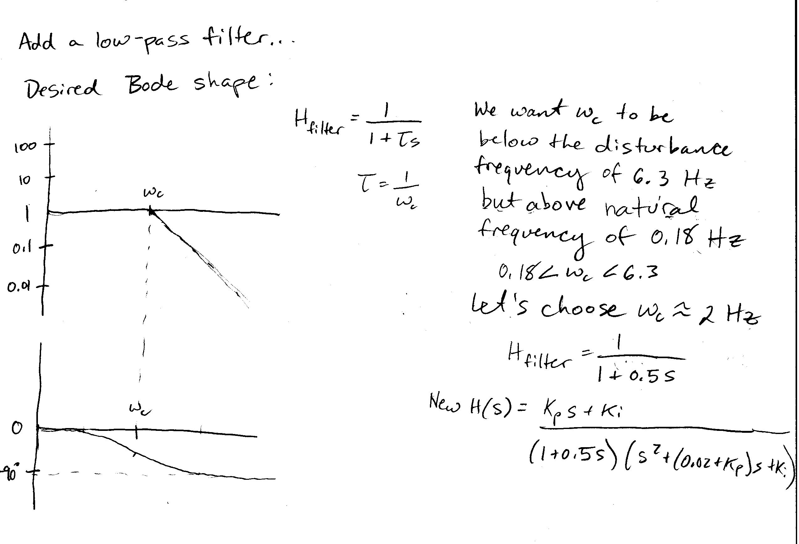
The PI controller proved effective in achieving our design goals when the disturbance input was a constant road angle of 60 degrees. However, when we varied the disturbance input to be a sine wave of frequency 6.3 Hz and amplitude of 60 degrees (simulating the conditions of a very bumpy, uneven road), our overshoot and rise time values no longer matched our design specs, so we adjusted our controller gains accordingly. Additionally, the steady state response oscillated between 59 mph and 61 mph. Although this deviation is not very great from our target value of 60 mph, there was also a resulting oscillation in controller effort, which is not ideal from an efficiency standpoint. Therefore we also added a low pass filter with a cutoff frequency of 2 Hz (chosen to be between the disturbance frequency of 6.3 Hz and the natural frequency of the system, 0.18 Hz). This filter in addition to the PI controller was effective in reducing the noise in the output velocity as well as the controller effort.
2. Mathematical Description
First Controller Design (for constant road angle)

With Kp = 0.2 and Ki = 0.0324
Second Controller Design (with low pass filter, adjusted for "bumpy" road)
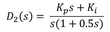
With Kp = 0.4 and Ki = 0.01
3. Block Diagrams
 Block diagram, PI controller, constant road angle step input


 Block diagram, PI controller, "bumpy" sinusoidal road input


 Block diagram, PI controller and low pass filter, "bumpy" sinusoidal road input


4. Design Derivation
First we determined that we needed to add an integrator to our transfer function to eliminate steady state error with respect to a step controller input as well as disturbance input...
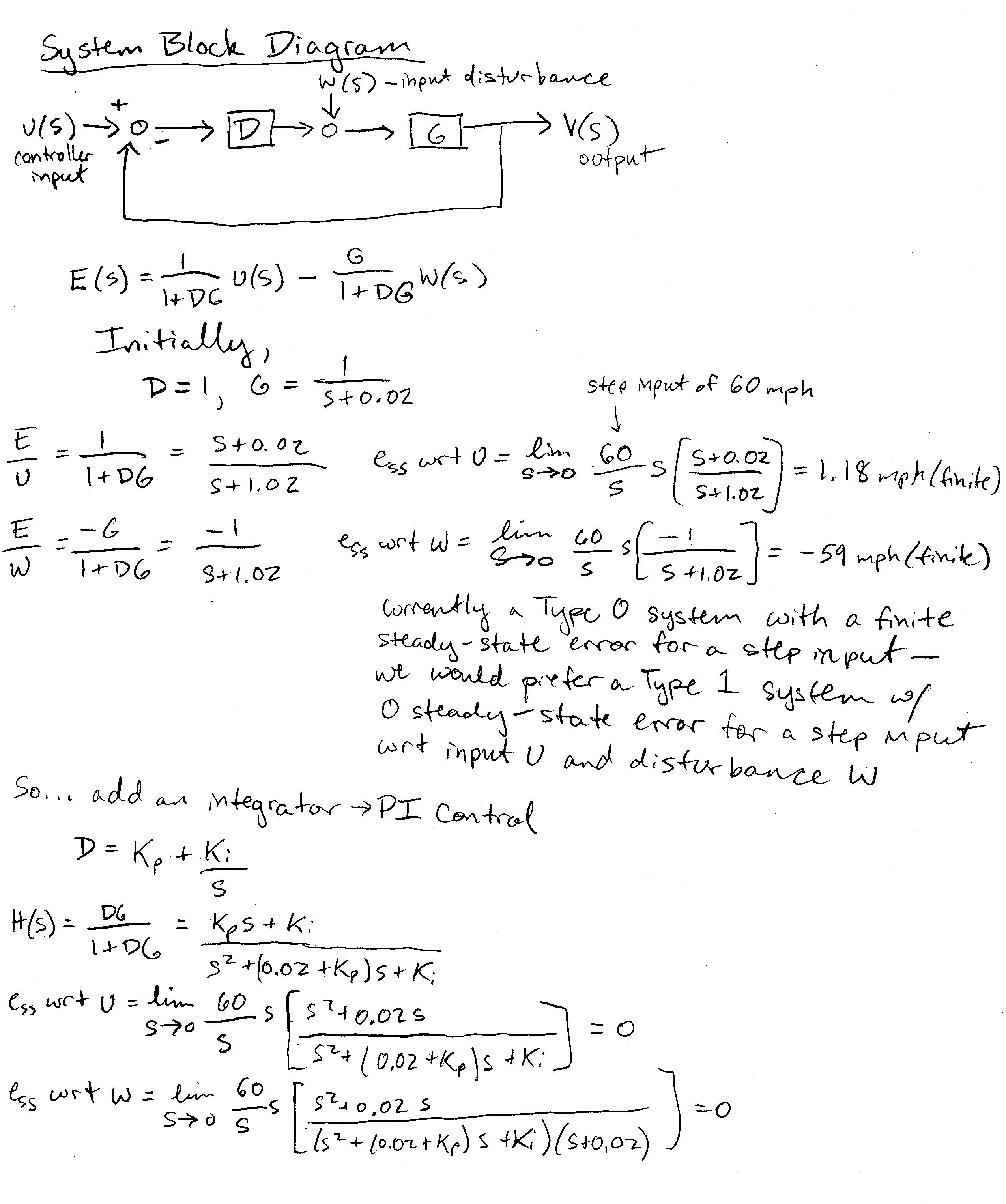
Next, we determined appropriate values of Kp and Ki based on our design specs (rise time around 10 seconds, overshoot no more than 8%)
The PI controller alone worked well when the road angle was constant, however a "bumpy" sinusoidal road angle function threw off our design specs, as well as caused an oscillatory controller effort. We tweaked our gains to Kp = 0.4 and Ki = 0.01 to shrink overshoot and increase rise time back to our desired values. Then we added a low pass filter to flatten out some of the oscillation in the steady state response.
Results
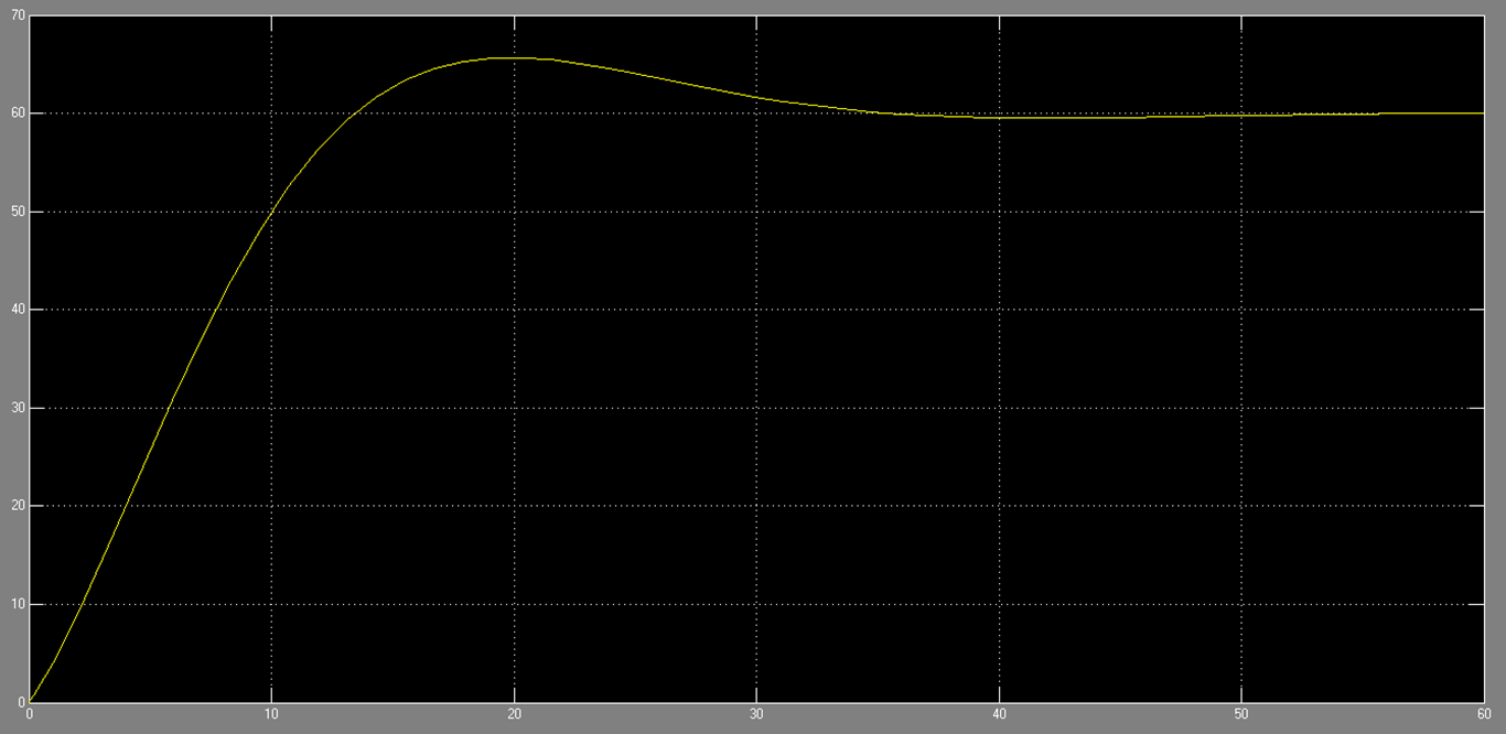
System response to step input 60 mph, constant road angle 60 deg, using PI controller
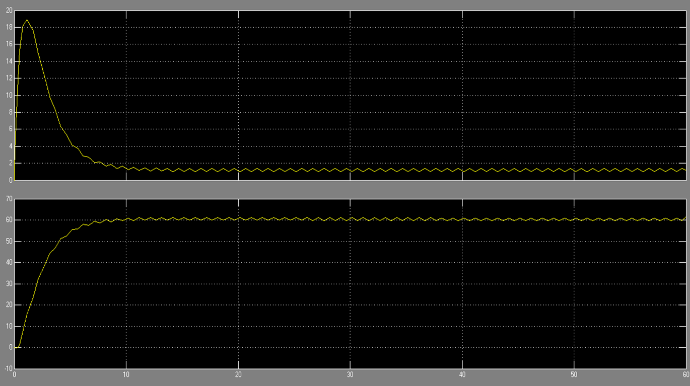
 System response to step input 60 mph, "bumpy" road input, using PI controller
  Above: Controller Effort
  Below: Output Response

 System response to step input 60 mph, "bumpy" road input, using PI controller and low pass filter
  Above: Controller Effort
  Below: Output Response
Conclusions
Adding a PI controller to the moving vehicle "plant" was extremely effective in reducing steady state error and meeting our design specifications for overshoot and rise time for a constant road angle. We can conclude, then, that when road angle changes gradually, our first design (D1) would be satisfactory in producing the desired system response. For the case of a very bumpy, nonlinear road angle, the gains had to be adjusted by inspection, and a low pass filter was added to reduce some of the variation in the system response and controller effort. In the future, the effect that the nonlinear bumpy road input has on the system could be examined more closely so that gains could be chosen analytically rather than simply by eye from looking at the system response to the nonlinear input in Simulink. Additionally, the use of a lead/lag compensator in place of a PI controller could be investigated to see if one is more suitable for this particular application.
Acknowledgments
Special thanks to Adam, Tania and Kirsten for helping us refine our project topic and understand our system! Also, thanks to Allison for teaching us about controls!
Files
Attach:Neville_simulink_models.zip
References
http://www.cds.caltech.edu/~murray/courses/cds101/fa02/caltech/astrom-ch4.pdf
Wiki examplesAttach:file.ext
Here is how to link to a file (note that you may need to compress/zip your code and CAD files into zip files so that that wiki will let you upload them, due to file type restrictions): Attach:HapkitTest.ino.zip
Here is how to add an image: 
Here is how to attach an image with the height adjusted (to 100 pixels)
Here is how to attach an image with the width adjusted (to 200 pixels)
Here is how to link a youtube video: