An Analysis of Liftware:

A look into control design for utensils that help people with tremor

---

Project team member(s): Brian Lozano and Michelle Warner

Abstract

For those with hand tremors, eating can pose a serious challenge. Liftware (a company purchased by Google) came up with a solution to this problem by creating a set of utensils that actively cancel out the tremor. According to their website, it works best for people with mild to moderate tremor (or tremors with a frequency between 4 to 12 Hz). In our project we looked at how to design a controller that would accomplish this task.

We decided to model our system as a translational system rather than as a rotational system. This greatly simplified analysis and is still a valid assumption because of the small amounts of movement that the spoon experiences. Additionally, we imagined our system to be a stationary one, rather than a moving one. What I mean by this is, the user is trying to hold the spoon stationary but cannot actually hold the spoon stationary because of tremor. What this means is desired movement of the spoon is zero and the controller will actively work to counter the movements due to tremor.

After creating our simple model of the plant, we used a PD controller to look at control methods. It's a fairly easy system to control and we found controller values to give us the desired results. Additionally we looked at the effects of using digital control and found a minimum time step at which control was possible.

Advanced Feature: We looked into the effects of digital control on the system

Introduction

The ability to eat independently is a skill that many people with hand tremor loose over time. This is degrading and makes dealing with the tremor even more embarrassing and public. A start-up called Liftware developed a discrete, portable and non-invasive solution to this problem in the form of utensils that use motors to actively cancel out the shaking from the tremor. As you can see in the video below, the product is remarkably effective. You can read more about Liftware's product on their website, given at the bottom of this site. The elegant implementation of controls and the obvious benefit for the users, make for a really interesting and tangible application of control design.

Liftware's Video really shows what a difference their product makes to users: https://www.youtube.com/watch?v=fS01kn6YJ94

Plant Model

We decided to model the system as a forced oscillating mass with the mass being the spoon. We did this because the spoon is mainly subject to lateral oscillations from the tremor, which can be modeled with a sinusoidal force. We chose to simplify the problem from angular displacements to a single lateral displacement because the tremors only displace the spoon by a small angle (measured from the elbow), which allows us to employ the small angle approximation and control for the displacement of the spoon, rather than its position based on the angle of the arm. This formulation still allows the tremors to be brought to zero and for the spoon to be usable because it cancels out the local vibration without removing the macroscopic movement of the arm.

Our Plant Diagram:

• Time Domain Equation:

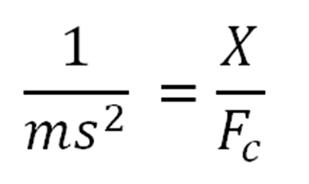
• Laplace Domain Equation:

Taking the tremor force as a disturbance, we ended up with a Laplace Equation of

• Model Parameters and Estimation:

• Simulink Simulation, Block Diagram and Results:

We decided to look at all results together in the Results section

Control Design

We ended up going with a simple PD controller. We were originally going to use to use a PID controller but in the tuning process we realized the integrator portion of the controller had no effect on our ability to achieve adequate control. Once we had our PD controller tuned we looked at the outputs of a continuous controller versus the outputs on a discrete controller. We found that the PD controller does an adequate job until the time step exceeds .003s after which the output goes unstable.

Continuous Controller:

Digital Controller:

Closed Loop Block Diagram:

Our block diagram includes the continuous controller on top and the discrete controller on bottom. Both the controlling force and output position are plotted on the scopes on top and bottom.

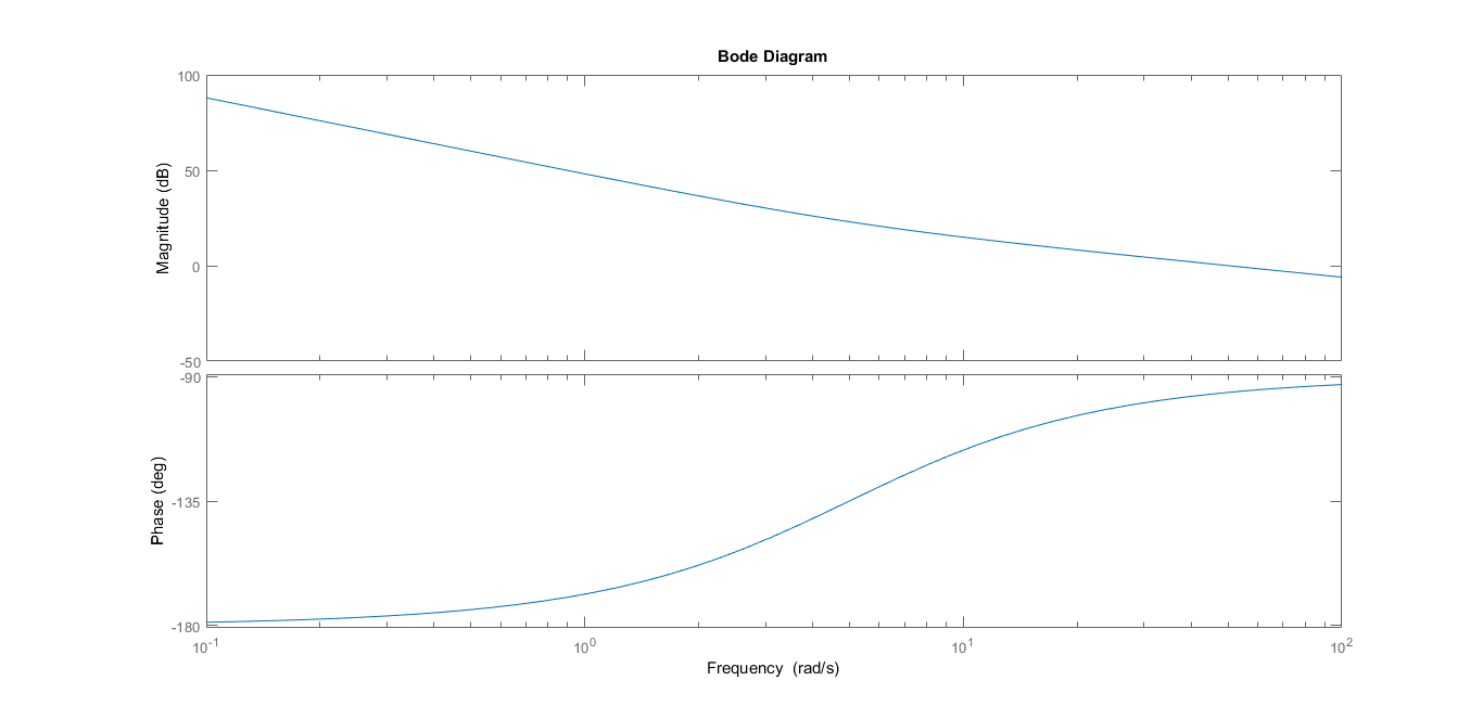
To tune the controller we started by looking at the open loop bode and root locus plots of the system. From these plots we can see that the output is oscillatory by nature and that there are two poles at the origin. In open loop both poles move up and down the imaginary axis. So our goal is to pull them away from the imaginary axis by adding a zero to the real axis in the LHP. The result is the closed loop root locus. We chose a ratio of Kp to Kd of 5, which then yielded the PD controller of K(s+5). By studying the root locus we decided on a K of 10. This makes Kp = 50, and Kd = 10. We also looked at the Root Locus of a PID controller but, we realized that the I term wasn't necessary and was possibly detrimental. The integrator term adds an additional pole to the origin and a zero very close to the origin. This actually forces the other two zero poles to venture slightly into the RHP before returning to the LHP. Thus, we eliminated integral control from the model. Our Bode plots of the open and closed loop system confirmed that we improved the stability of the system as we increased phase margin from 0 to 83.4 degrees.

Open Loop System:

Closed Loop Root Locus - PID

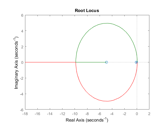
Closed Loop Root Locus - PD

Results

The Simulink model in the above section represents the closed loop system of the spoon, controller, and input sinusoid. This model is used to calculate the open and closed loop responses and control effort for both the continuous and digital systems over 1 second, which are shown below.

This system takes in both the oscillations from the sinusoidal forcing and an initial condition on velocity (meant to model the person picking up the spoon or reinitializing it). As seen in the open loop response, with an initial velocity the displacement of the spoon is not stable. The displacement continues to have large oscillations and to increase with an average velocity of the initial velocity.

Adding the PID controller and closing the loop brings the response under control and dampens the oscillations and initial velocity. As seen in the closed loop responses, the largest control effort is exerted in the first 1/10th of a second. The peak control effort is not much larger than that of the steady-state sinusoid control effort (-1.8 N as opposed to 1.1 N S.S. amplitude) after the initial velocity's influence has been removed from the error signal. The steady state sinusoid of the displacement has an amplitude of just over 2mm, which is very close to 0 when compared relative to the size of the spoon. As expected, the controller does not change the period of oscillation (8 Hz oscillation), but does greatly reduce the amplitude of the tremor's perturbation. Because the input signal is a sinusoid, the system never reaches a zero steady state error and instead reaches a steady state sinusoid.

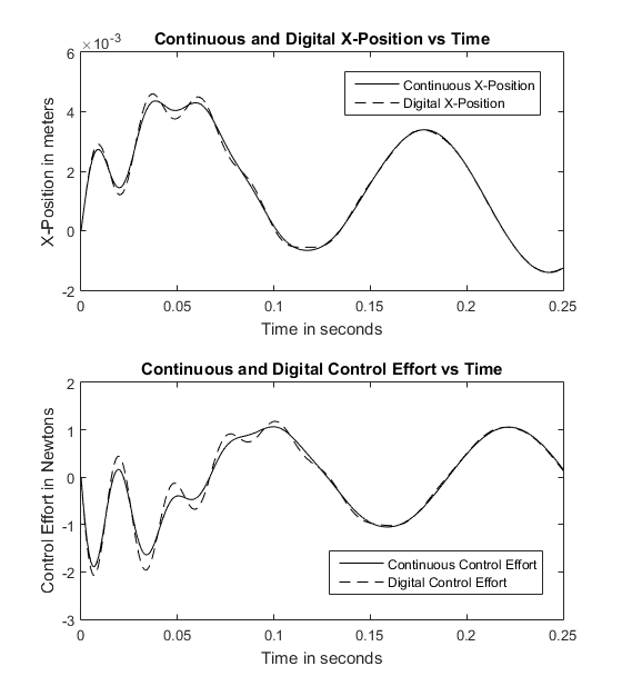
In the Simulink block diagram above, the lower of the two closed loop systems is a digital version of the upper continuous closed loop system. In the first set of closed loop responses below, the digital system response can be seen as the dashed line overlaid on the solid lines of the continuous response. It is worth noting that even with a satisfactory sample time (0.001 sec) the responses for both position and control effort of the digital system overshoot the peaks and troughs of the continuous system response. This is due to the time step between changes in the states, and changes in the error signal of the digital system which causes these overshoots after fast changes in the continuous response. This lack of accuracy due to a time sample resolution that is not fine enough is called aliasing. For a sample time of 0.001 seconds, the steady state values of the digital responses match those of the continuous responses.

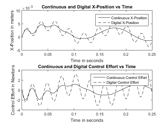
When the value of the sampling time is increased to 0.00215 seconds, the digital response gains much more aliasing which causes it to have a high frequency high amplitude oscillation when compared to the continuous response (as seen in the second set of responses below). This again comes from the digital system's inability to track the dynamics of the system because its sampling frequency is too low. As sampling time is increased even more, the system becomes less and less stable until the point where it diverges and becomes completely unstable. This shows the importance of choosing an appropriate sampling time when dealing with digital control systems. In the case of this project, a sample time at or below 0.001 seconds yields satisfactory system dynamics.

Conclusions

Overall we managed to come to a satisfactory level of control over our model. However, we made a lot of simplifications in the model and are unsure of whether or not, this solution would work in practice. The main assumptions that may not be valid are: (1) motion occurs predominantly in one direction and motion in the other two directions can be neglected and (2) we simplified the motion to be translational rather than rotational to keep our equations as simple as possible. If we had had more time we would have liked to develop a rotational based model in the form of a distributed-mass double pendulum. We spent considerable time trying to make this work but this model is really out of the scope of the class. This would have considered motion in two directions rather than one and been a more accurate representation of how joints move.

Files

Attach:WarnerLozano_MatlabAnalysisScript

Attach:WarnerLozano_SimulinkClosedLoopControl

Attach:WarnerLozano_Plots1

Attach:WarnerLozano_Plots2

Attach:WarnerLozano_Plots3

References