Submarine buoyancy control

Project team member(s): Mike Carter and Sae Yong Jang

Abstract

In this analysis we develop a model for the dynamics of a submarine's depth underwater as actuated by its ballast tanks. Submarines manipulate their buoyancy force by controlling the amount of air and water in these tanks. Our plant model includes non-linear effects such as fluid drag, which depends on velocity-squared, and saturation effects such as constraints on ballast volume and the fact that buoyancy only applies when the submarine is underwater. After developing this model, we approximate all of the non-linear aspects with linear models in order to derive a transfer function, and use classical control design tools to tune a controller that stabilizes the system's response to step inputs of depth. After completing this linear analysis, we include a less rigorously-derived but equally capable controller that works on non-linear plant dynamics.

Advanced Feature: Simulink model of the nonlinear system

Introduction

We plan to investigate and understand the control systems involved in piloting a submarine at desired depths. In brainstorming project topics, we both agreed that we wanted to look at a system that was unlike any of the examples we had seen in class so far, so that we could practice applying the skills and control techniques that we have learned in any context. As a result, we avoided the common topics and thought creatively. As an aquatic athlete, Mike has always been fascinated by the challenges of movement through the unfamiliar medium of water, and the extra forces that come into play such as buoyancy and non-trivial drag. We decided that it would be an interesting challenge to understand how a submarine controls its depth through manipulation of buoyancy forces.

Submarines primarily rely on ballast tanks for depth control. These tanks are filled with air from compressed air reservoirs on-board the submarine when the submarine wants to ascend and surface, and they are filled with water from the surrounding ocean when the submarine wants to submerge. It is a simple but effective way of changing buoyancy and controlling depth. Real submarines also have hydrofoils that act like wings when the sub is moving forward, generating a lift force, but we plan to neglect these in our analysis and focus on the ballast tanks as the primary method of controlling depth.

Plant Model

In order to determine a strategy for controlling our submarine's depth, we need to develop a model for the plant, or the dynamics that govern the motion of the submarine in its environment. As we mentioned, submarines manipulate their position underwater by adjusting the buoyancy force provided by ballast tanks on-board the vessel, as well as by generating lift forces with hydroplanes. Our analysis will ignore the hydroplanes because they act via the submarine's forward velocity, which open's the system up to an additional dimension and a host of other control goals. Instead, we will restrict our focus to the primary actuator for depth control - the ballast tanks. We define our plant to include the submarine underwater, actuated by manipulation of airflow into/out of the ballast tanks.

The submarine sinks by letting water flow into the ballast tanks and, and air flow out of the tanks. It gains buoyancy by filling the tanks from on-board compressed air reservoirs. We will model this control input by assuming we can set a specific volumetric flow rate of air/water into/out of the tanks. We could imagine this to be feasibly implemented by adjusting flow regulation valves on the compressed air lines (for air inflow), or by adjusting the ballast tank outflow gates to vary flow areas. We define air flowing INTO the tank as positive volumetric flow, and we will assume that the total volume of the ballast tanks remains constant. We also define the variable x to refer to the submarine's depth. Note that this means an increasing x corresponds to submarine sinking. We will further assume that variation in the pressure and density of the water immediately surrounding the submarine is very small compared to the variation of pressures at different depths that the sub could explore.

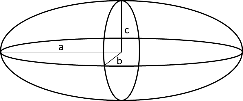
In developing our plant model, we are trying to faithfully recreate the forces and dynamics involves in submarine depth determination. This means we are allowing our system to exhibit non-linearities. There are three forces that act on the submarine in the vertical direction. There is a constant gravitational force that acts on the dry mass of the submarine. We use the term dry mass to refer to any mass that is not used in the ballast system. In real submarines, sometime fuel tanks are considered in the ballast mass because they will be changing. We are assuming that our fuel mass remains constant, and is contained in our "dry mass". Second, we have a buoyancy force that always acts in the direction of decreasing depth. This force depends on the volume of air in the ballast tanks. The buoyancy force can be derived from a force analysis of a control column of water, which gives a simple and intuitive result. The force is equal to the difference in weight between the water that is displaced by the container, and the weight of the fluid (air) that fills the container. Finally, we have a fluid drag force. Note that this force depends on the square of the submarine's velocity, so it is certainly non-linear. We used the drag coefficient of an ellipsoid to approximate the form of a submarine, and used metrics of a real naval submarine for all of our parameters.

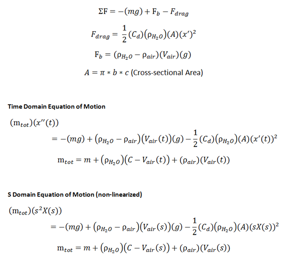
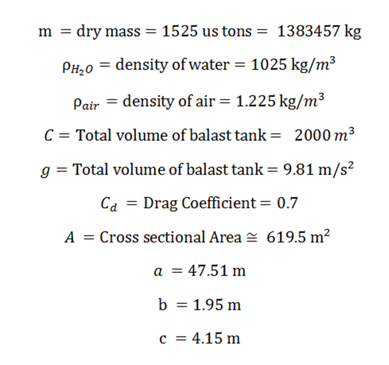
• a,b,c,m, and C are belong to USS Gato Class specification
• Cd is estimated from the ratio of (2b)/(2c) = 2 (estimated)
• A, surface area of ellipsoid, is estimated by using the equation above

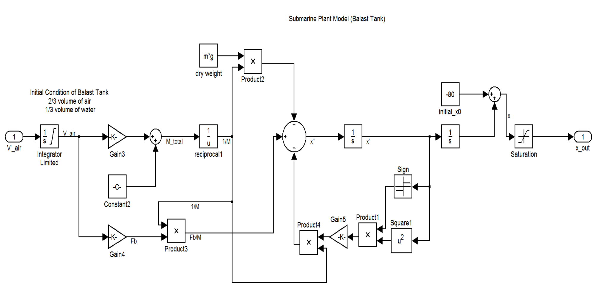
Having formulated the plant equations that govern the depth of the submarine, we built a simulink model of the open-loop system. The model reflects all of the non-linearities that we identified in our system. We were careful to preserve the sign of x' when squaring it to be sure that the force acted in the appropriate direction. We also implemented some logic controls to be sure that when the sub reaches the surface, the buoyancy force ceases to exist (the sub does not float into the air). We also limited the integration of our control input, V'_air, so that the total volume of air in the ballast tanks cannot excede the capacity of the tanks.

• Non-linearized Submarine Plant Model

• Open-Loop System Result for depth over time

We can see that without closing the loop on our depth control system, a positive step in volumetric air flow rate (increase in air inflow to ballast tanks) results in an uncontrolled upheaval to the surface. To mimic the real system, we limit the range of x to be always negative since submarine will not behave like a skyrocket. In order to correctly control the depth of our submarine, we will need to develop some kind of feedback control structure around this plant.

Control Design

In order to use the tools we have learned in E105, we need to be able to model a system with its transfer function. Since our plant model is non-linear, we cannot take the laplace transform, and as a result we cannot generate a transfer function to relate volumetric flow rate of air to submarine depth. To use tools like root-locus analysis, we will linearize our plant model and represent this approximation with a closed loop transfer function and a PD controller. We assume a starting condition of neutral buoyancy so that we do not have to deal with the constant gravitational term in our transfer function, and thus we define any change in the buoyancy force to be relative to this condition in which the buoyancy balances the weight of the sub. We also linearize our drag function with the assumption that (x')^2 can be approximated by (x') for the range of speeds that we are likely to see. Moreover, since M_total is a function of time, we simply assume that M_total equals dry mass of submarine (constant value) in order to linearize the system.

With these simplifications, we are able to solve for the transfer function that related submarine depth to volumetric flow rate of air into the ballast tanks.

Now that we have our transfer function, we can use a root locus analysis to develop a well-tuned PD controller.

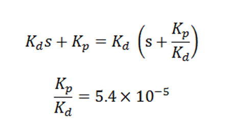
The poles of hte closed-loop transfer function must stay in the left half of the s-plane for the system to be stable. Therefore, we try to implement a PD controller by adding a zero, (Kp / Kd), at 5.4e-5 (close to the Imaginary axis). The zero contributes 90 degree of phase to change departing angle of the poles at s=0. Moreover, the zero changes the asymptote angles and alpha (the starting point of the asymptote lines). By manipulating the single gain value of Kd, we can design our controller to meet the system requirements. A root locus plot shows that we achieve stability by implementing the following PD controller. Kp = 5.4e-7 and Kd = 0.01. At Kd = 0.01, the poles are located at -0.00292 + 1.1 i and -0.00292 -1.1 i. The natural frequency is the magnitude of the poles, and it is about 1.1 rad/s. Unfortunately we cannot use the equations we learned in class to design for a specific rise time and overshoot since our system is not well approximated as second order, and the damping ratio varies widely from 0.5. Instead, we have used the PID tuner in MATLAB to meet time the following domain requirements: Rise time = 200 s and overshoot = less than 15%.

Results

Having developed our new controller, we were eager to test it in simulation. We found the following results.

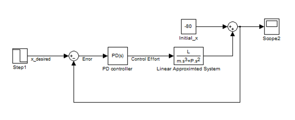
• Closed-loop Linear System Response to a Step Input

We notice that the settling time is longer in our system than it would be in real life. In a real submarine system, the submarine manipulates its screw turbines, pitch angles, and the angles of attack of its hydrofoils to get extra control over its dynamics; It does not rely solely on its ballast tanks. A more complex model that included thes other actuators would likely be able to predict more accurately the dynamics and response of the submarine system to depth control inputs.

We were excited to have developed a controller that stabilized our linearized model of the submarine system. However, we were somewhat dissatisfied by the extent to which we had to fudge and approximate our model in order to use the tools we learned for linear systems in E105.

We tried to use Kp and Kd values approximated from linearized model to our non-linear model. However, it did not work greatly for the non-linear plant model.

• Non-linear Submarine Plant Model with Closed Loop PD Controller

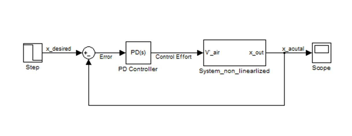
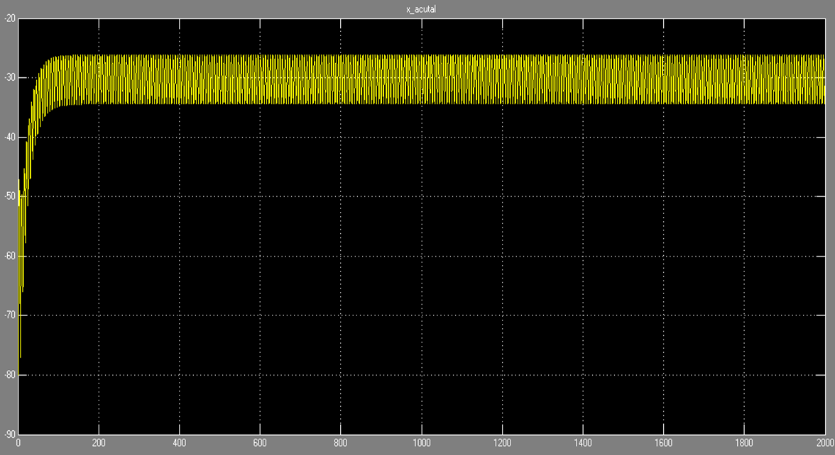
• Closed-loop Non-Linear System Response to a Step Input (Kp = 5.4e-007, Kd = 0.01)

As shown above, PD controller was not working properly due to difference between non-linear and linear approximated model.

We made an attempt at implementing a second PD controller around our non-linear plant model. With a little bit of intuition, patience, and trial-and-error, we were able to successfully tune this controller to give us a very reasonable response even on our non-linear plant. By setting Kp to 3 and Kd to 55, we notice that it shows reasonable result, although it is not stable by oscillating around desired position depth.

• Closed-loop Non-Linear System Response to a Step Input - Float (Kp = 3, Kd = 55)

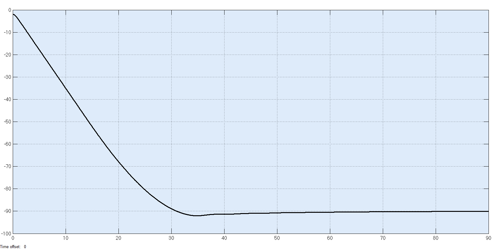
We also tried Kp = 3 and Kd = 55 for non-linear plant diving scenario. we are able to make our submarine dive from the surface to 90m of depth in about 30 seconds with little only a couple of meters of overshoot and zero steady-state error. This step input corresponds to an interesting real-life dive scenario for naval submarines. In maritime warfare, submarines have a tactical advantage; they can take cover from aerial threats underneath the water's surface. Naval subs can perform a maneuver called a "Crash Dive", which is an emergency evasion technique to escape a threat at the surface of the water. A fully-crewed submarine can dive to a depth of 70-90 meters in approximately half a minute. Here we use our non-linear PID controller to demonstrate the execution of a crash dive from the water's surface to the desired cover depth of 90 meters.

• Closed-loop Non-Linear System Response to a Step Input - Dive (Kp = 3, Kd = 55)

Conclusions

In this analysis we have presented two controllers that stabilize the dynamics and response of a closed-loop depth control system for a submarine. We used classical design tools in our first controller to tune gain parameters around a linear approximation of our system. We achieved satisfactory rise-times and overshoot values, however we noticed that under some circumstances the system had a longer settling time than we would have liked. We were also able to tune a PD controller to give very satisfactory response results around the non-linear system. In fact, this controller generally performed better than the one we developed for the linear model. Unfortunately, the results from linearized and non-linear model are different from what we expected due to limitation of approximation.
However, it worked so well that we could replicate a fairly advanced naval submarine maneuver, known as a "Crash Dive".Given more time we would love to upgrade our model and our system to address the other dimensions and actuators on a submarine, such as the forward velocity and the corresponding lift force generated by hydrofoils and pitch angles. Also, we can find better method to deal with non-linear model tuning. This kind of MIMO system was far beyond the scope of this mini-project, but it would be very interesting to explore the interplay between different actuation effects.

Acknowledgments

We would like to thank Adam for his guidance through this project, and the helpful world of submarine enthusiasts for providing background information that was critical to our ability to understand and analyze this interesting topic.

Files

Attach:Carter_Jang_Simulink_Model_variables.zip

Attach:Carter_Jang_Simulink_Model_float.zip

Attach:Carter_Jang_Simulink_Model_dive.zip

References

Attach:Matej.pdf Matej, David. Global Maritime Transport and Ballast Water Management. PDF available:

http://maritime.org/doc/fleetsub/chap4.htm

https://en.wikipedia.org/wiki/Submarine

https://en.wikipedia.org/wiki/Ballast_tank

https://en.wikipedia.org/wiki/Crash_dive

---