

Phillip Giliver Chris Cruise

Active Aero In Action:
The McLaren P1's spoiler changes
its angle of attack to maximize
downforce at the wheels.
Active Aerodynamics/Suspension Deflection on Sportscar
Project team member(s): Phillip Giliver and Chris Cruise
Abstract
In the automotive industry, the advent of computer control has allowed for higher performance, safety, and comfort for various types of vehicles. One technology that many high-performance manufacturers are exploring is active aerodynamics, in which a vehicle's aerodynamic properties are adjusted based on a desired vehicle behavior. This adjustment is performed either through a set of hydraulically, pneumatically, or electro-mechanically driven aerodynamic flaps. For our project, we are considering an electro-mechanical spoiler (as per the new Porsche 911) that is settling the rear of a decelerating vehicle. By controlling the torque on the aerodynamic flap, we are aiming to stabilize the tire traction at a particular value. Our plant consists of both the aerodynamics of the spoiler as well as the vehicle suspension dynamics because ultimately, the point of the active aero is to provide the car with additional traction. Physically, our control goal was to provide the desired amount of downforce as quickly as possible, and then not oscillate about the set point. This is to generate too much traction for most of the transient response to ensure that the car does not go unstable due to a lack of traction. The final controller was a double notch compensator, which yielded a step response rise time of 0.4s and settling time of 0.6s - approximately the same as the Bugatti Veyron.
Since we are looking at the dynamics of an electric motor, aerodynamics system, suspension deflection, and then tire deflection, our plant transfer function was of order four. This order resulting from a second order aerodynamic system from Torque to Downforce and then a second order spring-mass-damper suspension system from Downforce at the spoiler to Normal Force at the wheel. Tractive Force was then a constant coefficient of friction multiplied by this Normal Force.
Introduction
This project was inspired by the active aerodynamic system implemented on the Pagani Huayra sportscar [1]. This vehicle uses four electromechanically actuated flaps similar to ailerons on an aircraft to actively control downforce. Similar active aerodynamic implementations exist on Porsche 2014 911 Turbo (active rear spoiler) and the Bugatti Veyron (active flaps and vents) [2]. The previous state of the art used active suspension to adjust the vehicle dynamics which provides some level of control over downforce as well. Active aero systems improve upon this design (although both methods are typically implemented together) in that the high level vehicle controller can demand downforces directly without otherwise affecting the vehicle dynamics. For this project, we will focus on the Porsche and Bugatti implementations to control a single actively actuated airfoil at the rear of a vehicle to provide traction to rear wheels. The key element of this system is the relationship between downforce and airfoil angle of attack [3].
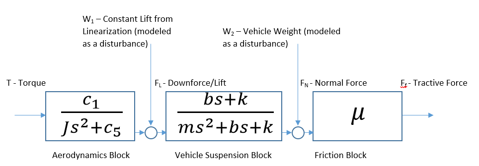
Plant Model
Overall, the plant starts at a torque provided by a motor to control the angle of attack of a car spoiler. This provides a downforce that is transferred through the car suspension, modeled as a spring-mass-damper system, to the wheel to provide a demanded tractive force. We broke this plant into two major subcomponents � the aerodynamics of the spoiler and the vehicle dynamics of the suspension system. The aerodynamics relate the downforce provided by the spoiler at a certain angle of attack to the torque required by the motor to maintain that angle. To generate more downforce, the motor must provide more torque to increase the angle of attack of the spoiler. Once the downforce is calculated, it is used as an input to the vehicle dynamics component. The vehicle dynamics were modeled as a spring-mass-damper system with an input downforce and an output normal force that is seen at the wheel. The tractive force from here is simply the product of the coefficient of friction between the wheel and road (assumed constant) and the normal force. The initial downforce resulting from the linearization of the aerodynamics and the weight of the vehicle, initially modeled as disturbances, each provide a constant tractive force as well. To remove their effects, the demanded signal is not for total traction, but for "additional" traction from a baseline traction (see derivation for further details).
For our model, we have three different transfer functions that describe the aerodynamics, spring-damper dynamics, and friction.
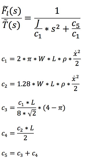
In the first model, we model an applied torque on an aerodynamic flap and the resulting downforce from the flap. From aerodynamics equations from [4] and [5], we find the following:

In the equation above, tau is applied torque, Fl is lift force (in our case lift is downwards), l2 is the horizontal distance to the centroid of the flap, Fd is drag force, l2 is the vertical distance to the centroid of the flap, J is the moment of intertia of the flap, alpha is angle of attack, W is the width of the flap, L is the length of the flap, rho is the density of the air, and x is the position of the vehicle.
To get rid of various constants (stemming from our linearization of the flap around a 45 degree angle of attack) in our derivation, we specified a nominal torque which maintains that angle of attack. After linearizing, we find the following transfer function:
In the second model, we model an applied force on a two-mass spring damper system. When the second mass is fixed, we find the following equations of motion for the two masses.

In the equation above, x is the displacement of the mass, m is the corner weight of the vehicle, k is the spring rate for the suspension, and b is the damping in suspension.
Finding the transfer functions for each of these equations of motion, we cancel X(s) to find the following transfer function:
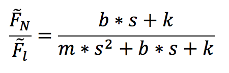
Finally, we multiplied our output force on the second mass (Fnormal) by a friction coefficient to obtain our desired tractive force.
The transfer function is the following:

All together, our open loop transfer function is the following:
Initially, we had constant terms of downforce from our linearization about pi/4 and the vehicle weight that could not be absorbed into the transfer function. These can be modeled as disturbances in the overall system.
Ultimately, we decided to only control additional tractive force to effectively ignore the constant torque/tractive force that these disturbances introduce into the system.

Attach:pg_cc_eom_derivation.pdf
| Parameter | Units | Value | Description | How Chosen |
| p (rho) | kg/m^3 | 1.225 | Air Density | Looked up at STP |
| L | m | 0.2 | Length of Airfoil | Average spoiler length |
| W | m | 0.75 | Width of Airfoil | Average car width divided by two (Spoiler width split to two wheels) |
| v, xdot | m/s | 40 | Vehicle Speed | Expected racecar speed ~ 100mph |
| a (alpha) | rad | Linearized at pi/4 | Angle of Attack | Halfway between min (0 rad) and max (pi/2 rad) spoiler angle. |
| J | kg-m^2 | 0.0133 | Mass Moment of Inertia of Spoiler | Calculated from L, W and spoiler mass of 3kg |
| k | N/m | 80,000 | Spring Constant | Looked up for average vehicle [6] |
| b | N-s/m | 350 | Damping Constant | Looked up for average vehicle [6] |
| u (mu) | Unitless | 0.7 | Coefficient of Friction | Looked up for standard, dry road conditions |
| m | kg | 375 | Vehicle Mass | Weight of car (1500kg) on one wheel |
| To | N-m | 67 | Motor Torque Offset T = T0 + T~ | Calculated using above parameters |
| Fl,o | N | 1920 | Downforce Offset Fl = Fl,o + Fl~ | Calculated using above parameters |
| FN,o | N | 5600 | Normal Force Offset FN = Fl,o + mg/4 + FN~ = FN,o + FN~ | Calculated using above parameters |
| Ff,o | N | 3900 | Ff,o = u*FN,o | Calculated using above parameters |
The following images show the step response of the entire plant with an input of motor torque and output of tractive force from 0 to 5s and until it decays:


Additionally, the following images show the step responses of the intermediate aerodynamic (input torque, output downforce) and suspension (input downforce, output normal force) step responses.


From these images, we see that the main issue of the open loop system is that it is incredibly underdamped. First off, the aerodynamic block has no damping at all (as can be easily seen by its transfer function) which causes it to pass a sinusoidal input into the suspension block which is underdamped. This leads to large sinusoidal output variations in tractive force in the short term. This sinusoidal response is unacceptable for this system because the vehicle's acceleration or deceleration is limited by the amount of traction available and if it ever tries to use more traction then the wheels will slip which can cause instability in the vehicle. This is likely in this open loop case since the amount of extra traction generated varies so greatly. Additionally, the system does not reach steady state for well over 60 seconds which is well beyond the time that it could possibly be useful to a car which needs the additional traction in real time.
Control Design
First, we decided to look at the open loop behavior of the system plant on a root-locus plot. Clearly, there are two sets of complex poles that we need to deal with. To deal with the poles near the imaginary axis that potentially could go unstable, we tried several different methods. Our target specifications can be found in the results section.
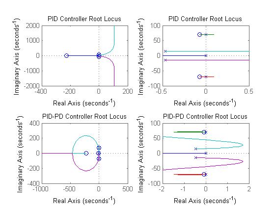
Initially, we attempted a PID controller, but found that it was only stable for a small range of overall gain values. This led to a limited ability to tune to meet system response specifications. To help with stability, we added an additional PD controller in series (a PID-PD) to add another zero to the system, which helped to bring the system to stability for all gains, but still could not be tuned to meet specifications.
Our final controller was a dual notch compensator design that brought the system to stability and was also able to be tuned to the system specs.
To add zeros in any location on the real axis, a PD controller of the form Kds + Kp can be used which creates a zero at -Kp/Kd. To add complex zeros, a PID is implemented of the form (Kds^2 + Kps + Ki)/s which has the added affect of creating a pole at the origin. The PID controller can create a double zero, a complex zero, or two distinct zeros. Effectively, the PID is Kd*(s+z1)*(s+z2)/s. The open loop plant has four poles and one zero, so we tried to add three zeros to bring the system to closed loop stability. The additional zeros were added near either the suspension complex poles or the aerodynamic complex poles. Overall, this attempt at a controller yielded the following result:

A notch compensator is of the form of:

This particular kind of compensator adds two complex zeros and two real, repeated poles. The zeros that come from the compensator can be accurately placed, and "cancel" the dangerous plant poles that could potentially go unstable. The following expression describes the location of a zero placed by the notch compensator:

Once we had solved a system of equations to determine our damping and natural frequency, we had our zeros and poles fully defined. The poles from the compensator were placed far enough on the left-half plane such that they did not present significant stability issues.

First, we began by considering the root locus of the plant by itself which is shown below along with a zoomed in image near the origin.
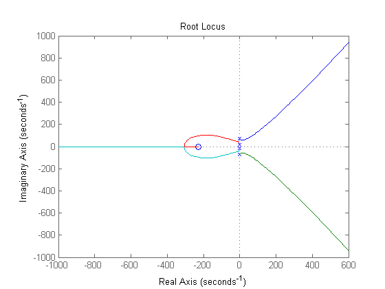

From these plots, we noted several important characteristics. First off, two poles were on the imaginary axis from the aerodynamic system which were never stable for any closed loop gain. Also, there were two complex poles from the underdamped suspension system, but these were stable in the closed loop system because they went to the very negative zero created by the suspension system as well. Overall, we needed to find a way to cancel out the poles near the imaginary axis for stability as well as trying to pull them towards the real axis to remove oscillatory effects. Initially, we tried adding complex zeros near the aerodynamic poles, but we found that the suspension poles tended to take over these zeros as the aerodynamic poles went to the suspension zero on the real axis.
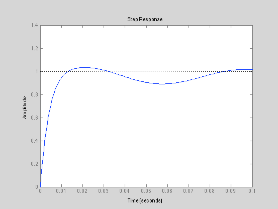
For the PID-PD series controller, we tried using zeros exclusively on the real axis to both decrease oscillatory affects and providing a means to achieve critical damping of the system. For most of our PID-PD controllers, we found that low gains went unstable from the aerodynamic poles crossing into the right half plane, but high gains were always stable after exiting that region. The major issue we found was that regardless of where we put the zeros, the system response was on the other of milliseconds instead of approximately 0.5s as we expected [7]. The reason that we rejected this response on the order of milliseconds is because that in the physical system, it is unrealistic for a motor to be able to generate the magnitude of force to create such an angular acceleration on the spoiler. To attempt to slow down the response, we always used near the minimum overall gains for which the system was still stable for a given controller which were obtained from the root locus plots. The following images show the root locus plots and step response for our attempted PID and PID-PD controllers:

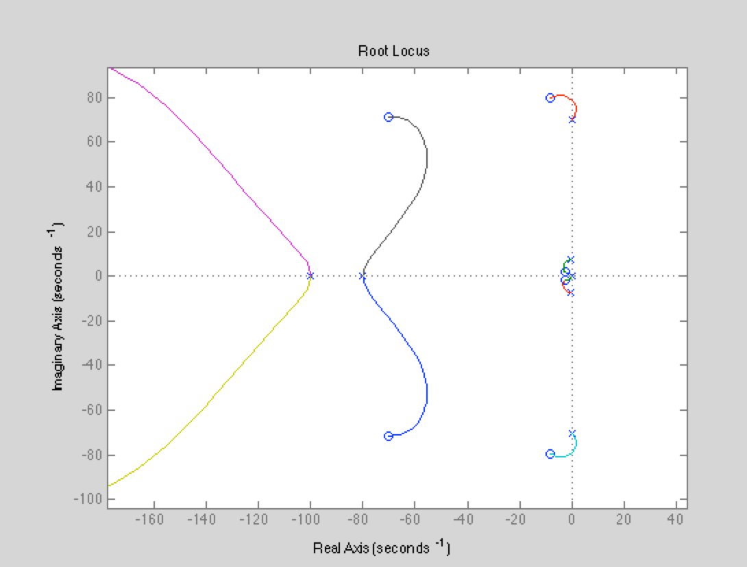
When first considering the possibility of using notch compensators to cancel out the unstable plant poles, we also added two PID controllers (in total 4 separate controllers!) to stabilize the added poles. For this PID-notch compensator series controller, we tried to place zeros near the unstable poles (by playing around with the damping and natural frequency values a bit randomly) on the imaginary axis. By doing so, however, we also placed a set of repeated poles on the real axis, causing other sources of instability. Ultimately, we were able to stabilize the plant poles, but the additional poles from the notch compensator caused the closed loop system to be unstable. Inelegantly, we were able to get rid of this instability by adding a set of PID controllers to our controller series. Even with this level of controller complexity, we encountered the same issue of an unreasonably fast rise time (even with an attenuated signal) as before. The following images show the root locus and step response plots for the PID-notch controller:
Seeing that the notch compensators managed to cancel the instability of the plant, we wondered whether we could more accurately place their zeros such that we would have enough gain margin to ensure stability. Deriving the expression for the zeros placed by a notch compensator, we placed them nearly on top of the unstable plant poles. For our two compensators the corresponding natural frequencies and zetas were the following:

The full controller (with the two notch compensators in series) had the following form:

Once we had determined the form of the final controller, we plotted the root locus of the closed loop system and saw the following:
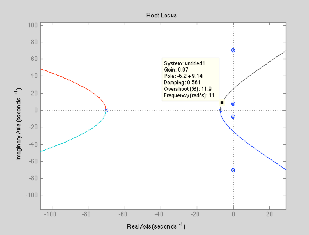
From this plot, we chose a feedback gain, and were able to meet our target specifications (see results section).
Results
After looking at the technical specifications for the Bugatti Veyron [7], we decided that our target system performance specifications would be similar. In the published press release, Bugatti claims that their air brake deploys in 0.4 seconds, which we set as our target rise time. Additionally, we decided that it would be preferable to demand slightly more downforce than required, but not less, for fear of having the vehicle lose traction. The downside to added downforce is a subsequent increase in longitudinal drag, so too much overshoot or steady state error (above the desired tractive force) would be undesirable as well. We decided to set a target maximum steady state error of +10%. And finally, we chose to specify settling time as well, to make sure that our system achieved steady state fairly quickly. This target settling time was chosen to be 1 second. This may seem like a long time, but we decided that since we never go below our target tractive force, the detriments of providing "too much" traction for some period of time before settling are minimal.
The following is a step response plot of our controlled system:

In this system, the input signal is the desired increase in tractive force and the output signal is the actual increase in tractive force. By inspection, the system seems to meet our specifications, but to verify we also checked the performance of the controlled system with the built-in MATLAB command stepinfo:

Conclusions
Given the target specifications we set, our system response is now satisfactory and realistic for a physical system. As seen in the results section, our rise time, steady-state error, and settling time were all within specifications. Additionally, with our previous controllers (PID-PD and PID-notch), we were able to stabilize the system, but with completely unrealistic rise times (on the order of 0.01 seconds). Now, however, our rise time is the same order of magnitude as the Bugatti Veyron's and feasible.
If we were to adjust our approach, we would likely model the system dynamics a bit more accurately (aero-flap motor damping, tire deflection, etc.) as this would attenuate the sinusoidal behavior in our system. Additionally, we could attempt to model the non-linear effects of the angle of attack-downforce relationship to better simulate true system behavior.
Files
This is the MATLAB script that plots the plant behavior (including only aerodynamic response and only suspension response), the root-locus for the final notch controller, and the time response for the final notch controller.
References
[1] https://www.youtube.com/watch?v=-_bakHYcD9o
[2] http://www.bbc.com/autos/story/20140819-carmakers-slippery-new-buzzword
[3] https://www.comsol.com/blogs/how-do-i-compute-lift-and-drag/
[4] https://www.grc.nasa.gov/www/K-12/airplane/kiteincl.html
[5] https://www.grc.nasa.gov/www/K-12/airplane/kiteaero.html
[6] http://ctms.engin.umich.edu/CTMS/index.php?example=Suspension§ion=SimulinkModeling
[7] http://www.bugatti.com/veyron/technology/