Balance Bot

Project team member(s): Robert Kobara, Allie Miller

Abstract

A balance bot is a two-wheeled robot that can maintain a vertical position even though this position is inherently unstable. The goal of this project is to design a controller for a balance bot that will turn the wheels of the robot at the correct speed and direction in order to counter its natural tipping motion. If designed correctly, the robot should return to a steady-state, upright position when subjected to an outside disturbance. Accelerometers are placed on the robot in order to measure the rotational deflection of the robot from its desired upright position. This rotation creates an error term that is used by a PID controller that outputs a torque to the motors to counteract the tilt and reduce the error to zero.

Because the microcontroller for this project works with digital signals, the system must digitized using Tustin Approximation. After performing simulations where the digitized system was subjected to an impulse disturbance while holding the reference tilt at 0, it was determined that the Tustin Approximation with a sampling period of 0.0021 seconds served as an accurate representation of the actual, continuous system. Additionally, it was determined that the PID controller modified the system such that it was stable when disturbed by a 0.1 Nm impulse torque about the wheels. However, in order to achieve this desired response, a motor that can output at lease 7 Nm of torque in response to the impulse must be used.

Advanced Feature

The advanced feature for this project is the use of digitization. This is implemented by taking samples from an accelerometer at a fixed sampling frequency. The accelerometer is rigidly attached to the robot and provides the instantaneous angular pitch of the robot at each discrete sampling point. These points, in turn, are used to create a digital position signal that is then used by the PID controller to actuate the motors so they can correct for any disturbance in the system position.

Introduction

For this project, the system under study is a simple robot that is meant to balance on two wheels in the face of small outside disturbances. The robot is equipped with an accelerometer that will sample the robot's tilt at a constant sampling frequency. This digital signal will be used by an on-board microprocessor that will create a control output of the motors that will stabilize the robot's tilt. Overall, the system will be very similar to this two wheel inverted balancing robot. The inspiration for the topic of this project was an encounter with a self balancing unicycle on campus. With this vehicle mind, along with the recent popularity of segways and hoverboards, it was determined that balance control is a relevant topic in today's technology, and this project provided the perfect opportunity to explore the topic further.

Plant Model

The system under study is a balance bot, which is a small robot supported by two wheels. Each wheel on the robot is controlled by a DC motor. Because there are only two wheels, the system is inherently unstable and any small disturbance to the balance of the system when no controller is present will cause the robot to tip over.

To analyze the balance bot system, we focused on the forces and torques inherent on each of the wheel motors and then derived the time-domain equation of motion for the balance bot from there. The important parameters that emerged from this method included the motor torque for each wheel, the torque present on each motor due to the robot's center of mass around the axis of rotation, friction, and inertia. A free-body diagram depicting the forces and torques on the motors can be seen below:

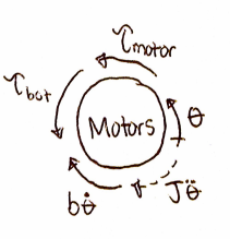
From this free-body diagram, the following equation of motion was derived:

This equation was then converted into the following Laplace-domain transfer function:

       θ/τ_motor =1/(Js^2+ bs-mgl)

The parameters that went into these models are as follows:

	b = friction/damping = 0.028 [Nms^2/rad]
	g = gravitational constant = 9.81 [m/s^2]
	J = motor inertia = 1.13 * 10^-2 [Nmsec/rad]
	l = distance from motor shaft to bot's center of gravity = 0.1 [m]
	m = balance bot's mass = 0.5 [kg]
	θ = bot's angle of rotation from the vertical [rad]
	τbot = torque on the motors due to the bot's mass [Nm]
	τmotor = torque the motor outputs [Nm]

The values used for these parameters came from multiple sources. For example, the friction/damping and motor inertia values came from the data sheet for a standard DC motor. On the other hand, the distance from the motor shaft to the bot's center of gravity, as well as the bot's mass, were estimated as what we think would be reasonable for a small balancing robot.

Finally, this equation of motion was used to create block diagram of the system as seen below:

An open loop analysis of the uncontrolled system was run using MATLAB. For the simulation, an impulse input was used to simulate a small disturbance equivalent to a 0.1 Nm torque about the motors. The resulting response (robot rotation about the wheel axis, theta) to the input was found to be as follows:

This behavior is extremely undesirable because it shows that when a small torque is applied, the resulting robot rotation quickly becomes unstable. This is equivalent to saying that the robot will fall over (large theta) when a small disturbance (small torque) is applied.

Control Design

We chose a PID controller because we wanted to eliminate steady-state error for the system while still achieving a physically plausible response time with minimal overshoot. Additionally, to make our controller physically realizable, we decided to digitize the system.

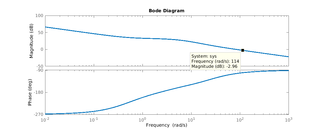
In order to digitize the system, a sampling period was needed. This period was calculated from the bandwidth of the system in question. The bandwidth was measured by graphing a Bode plot of the open-loop system and measuring the frequency that corresponded to -3dB (114 rad/s). It was determined that a sampling period of at least 25 times the bandwidth frequency would be sufficient for the Tustin Approximation method used to digitize the system. Thus, a sampling period of 0.0021 seconds (120 rad/s) was used.

The value for each control parameter was experimentally determined using closed-loop analysis on the plant-controller system. Each control parameter was adjusted and a 0.1 Nm torque impulse disturbance signal was applied to the closed-loop controller-plant system while holding the reference at 0. If the system went unstable, adjustments to the control parameters were made and another iteration of impulse disturbance testing occurred. The parameters were finalized after the steady-state value of theta became 0.

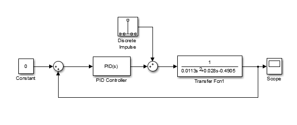
With all of this taken into account, the final controller design and the associated impulse response was set as follows:

Results

The closed-loop system with a 0.1 Nm impulse disturbance torque input was created in Matlab. It was determined that this torque was sufficient enough to represent small disturbances that the robot might encounter during normal use. Also of note, as seen in the Plant Model section, this impulse was sufficient to cause the open loop system to go unstable.

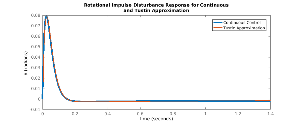
As seen in the following graph, the output of the simulation was the rotation of the robot (theta) in response to the disturbance. The blue plot represents the continuous, ideal closed loop response, while the red plot represents the response of the system that was digitized by Tustin Approximation method. Both plots follow a relatively similar path, with an initial spike of about 0.08 radians (about 5 degrees), followed by a decay to approximately 0 radians after about 0.2 seconds. This means that the impulse disturbances caused the robot to initially rotate approximately 0.08 radians from its upright position, but the motors created a counter torque that caused the robot to return to its initial position after approximately 0.2 seconds elapsed.

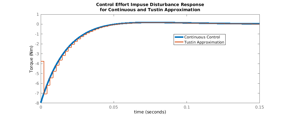
The graph below represents the control effort necessary to achieve the impulse output response described previously. Both the Tustin Approximation method and the continuous controller had similar shapes. In both cases, there was an initial spike of 7 Nm that decayed very quickly to 0. This meant that in order to get the rotational response to the disturbance impulse described earlier, the motors must provide about 7 Nm of torque.

Conclusions

As seen from the Rotational Impulse Disturbance Response plot and the Control Effort Impulse Disturbance Response plot, the Tustin Approximation method and the continuous control case are extremely similar. This means that the Tustin Approximation method provides an accurate representation for the controller and that the digitization of the system using this approximation should cause little to no negative impact on the controller. Additionally, the Impulse Output Response plot clearly shows that the robot initially rotates approximately 0.08 radians (about 5 degrees) from the upright position in response to the 0.1 Nm impulse disturbance signal and then proceeds to correct for this rotation and settles back at 0 degrees. This rejection of small external disturbances, while maintaining a vertical steady state position (0 degrees from upright) is exactly the behavior that is desired from the control system.

Even though this simulation clearly shows a valid proof of concept, there is still work that must be done. The most critical of these is the selection of the motors. As seen in the Control Effort Response plot, the motor must be able to provide 7 Nm of torque. A motor within the size and weight constraints probably cannot supply this amount torque. Thus, other possibilities must be explored. An example of an alternative is constructing a gearbox that can increase the torque transmitted to the wheels. Another option is performing experiments to explore the consequences of failing to reach this prescribed torque. Because this demand for high control effort occurs over a relatively short period of time (approximately 0.050 seconds), it is unlikely that the robot rotation will go unstable (i.e. the robot tips over) if the required torque is not met in that time frame. Therefore, the most likely consequence is that the insufficient motor torque will need to be applied longer to revert the robot to the desired, upright position. In other words, if the torque requirement is not met, the response will be slower.

Files

Attach:MillerKobaraOpenLoopAnalysis.zip: Matlab script used to run an open-loop 0.1 Nm Disturbance Impulse simulation on the plant.

Attach:MillerKobaraClosedLoopAnalysis.zip: Matlab script used to run a closed-loop 0.1 Nm Disturbance Impulse simulation with the plant and PID controller system.

Attach:MillerKobaraOpenLoopBode.zip: Matlab script used to create a Bode Plot for the open-loop plant and PID controller system.

Attach:MillerKobaraDigitalizedRotationImpulseResponse.zip: Matlab script used to run a closed-loop 0.1 Nm Disturbance Impulse simulation for the continuous control system and the Tustin Approximation with a sampling period of 0.0021 seconds, outputting the robot rotation from its upright position.

Attach:MillerKobaraDigitalizedControlEffortImpulseResponse.zip: Matlab script used to run a closed-loop 0.1 Nm Disturbance Impulse simulation for the continuous control system and the Tustin Approximation with a sampling period of 0.0021 seconds, outputting the control effort of the PID controller.

References

"Balanduino - Balancing Robot Kit." Balanduino - Balancing Robot Kit. Web. 04 Mar. 2016. <http://www.balanduino.com/>.

"SBU V3 (Self Balancing Unicycle)." YouTube. YouTube. Web. 04 Mar. 2016. <https://www.youtube.com/watch?v=Dev5NYzjRvk>.

"Two Wheel Inverted Balancing Robot." YouTube. YouTube. Web. 04 Mar. 2016. <https://www.youtube.com/watch?v=w6VqASRawgg>.

---