

Sammy Scaglione Sarah Cabreros Jose Lopez
Flywheel Feedback Control
Project team members: Sammy Scaglione, Sarah Cabreros, Jose Lopez
Abstract
This project examines a feedback control design of a flywheel shooting mechanism that Sammy and Sarah used for their final project in ME 210: Mechatronics. The system is comprised of a flywheel driven by a DC motor with an encoder. The DC motor is supplied with power and from the motor equations we know that this gives the attached wheel an angular velocity. This angular velocity, after some computation, can be determined by an encoder sensor. In chip shooting using a flywheel, final position of the poker chip often relies heavily on the angular velocity of the flywheel, and so implementing control to the system can increase the system reliability.
Advanced Feature: We will be incorporating time delay into our calculations.
Introduction
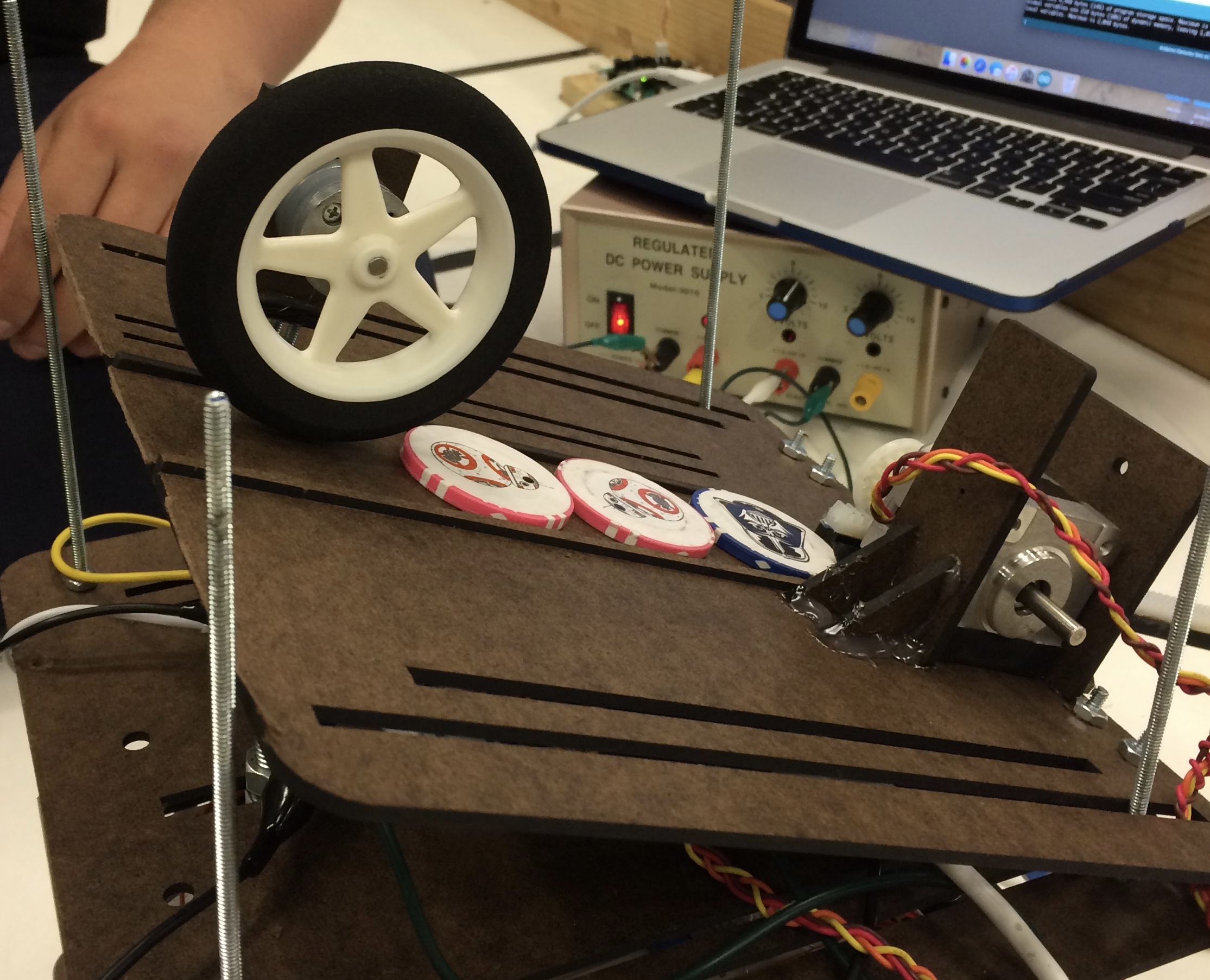
In its ME 210 implementation, the flywheel shooting mechanism is mounted onto a bot that shoots poker chips into buckets at various distances. The flywheel is run by a DC motor, whose angular velocity can be determined using an encoder. When a poker chip is fed underneath the rotating flywheel, the flywheel imparts linear momentum onto the poker chip, transferring in kinetic energy and thus an initial velocity onto it. This causes the chip to launch off the bot at a certain angle. By controlling the voltage supplied to the DC motor, we can control the angular velocity of the flywheel, which in turn controls the initial velocity of the launched poker chip. Given the group's strategy and the relatively large error margins of the ME 210 requirement with respect to final chip location, Sammy and Sarah did not implement any sort of control application of the flywheel. But what if Sammy and Sarah's group needed more precise position control? What sort of control over angular velocity could have been obtained if the project was given more than a short 3 weeks? Our group will use this project as an opportunity to explore these questions. We would like to reduce steady-state error to <1% and have a rise time t_r<1s. From this our group hopes to gain insight into how flywheel control can be done. Finally, we plan to incorporate time delay into our system. We did not get much practice with this important concept in class and so we will use it as an opportunity here to practice our learnings. This will leave us one step away from physical implementation of the controlled flywheel.
Plant Model
We seek to control a DC motor with attached flywheel to a certain tangential velocity. From this, our reference input is tangential flywheel velocity, which we can control using DC motor voltage. This DC motor voltage will produce a given output velocity.
Open-loop System Block Diagram:

We will now derive the transfer function for our plant.
Equation of Motion for Model:
V = iR + Kv*omega (1)
T_load = Km*i - Tf (2)
T_load = J*omega_dot (J = .5*m*r^2) and T_f = b*omega
Where,
- V is DC motor voltage
- i is DC motor current
- R is DC motor resistance
- Kv is the electrical motor constant
- omega is angular velocity of the flywheel
- T_load is load torque on the motor
- Km is mechanical motor constant
- Tf is internal motor friction
- J is flywheel moment of inertia about motor axis
- omega_dot is the time derivative of omega
- r is flywheel radius
- m is flywheel mass
- b damping constant
Substituting (2) into (1) we get,
Let's back out the tangential velocity at the edge of the flywheel, v = omega/r. This gives us,
Taking the Laplace transform of this equation, with V and v (voltage and velocity, respectively) as variables,
As a result, our overall system transfer function is
To put this in units of rad/s instead of RPM, we have to multiply by a factor of 30/pi.
To make the mathematics simpler, we define the following constants:
To proceed, we must now define all the constants included in these equations. Once we have done, this, we will be ready to design our controller for the system.
From the motor specs provided at https://www.pololu.com/product/2271 and the flywheel specs provided at http://www.rcdude.com/product-p/epw300.htm, we can deduce everything we need. We can get flywheel mass and radius from the latter link, and from the former, using rated 6V measurements, we get no-load speed, no-load current and stall torque.
At stall, omega = 0 and thus V=iR i.e. R = V/i. This will give us R.
At no-load we have V = i_noLoad*R + Kv*omega_noLoad (all of these values are provided). This will give us Kv
Finally, given Kv, we know Km = 9.5493e-3 * Kv, which given Kv is in units of V/kRPM we get Km in units of Nm/A. This will give us Kv.
| Km (Motor Torque Constant) | .053 Nm/A |
| R (Internal Resistance of the Motor) | .923 ohms |
| b (Damping Constant) | .1 |
| Kv (Motor Voltage Constant) | .0055 (rad/s)/V |
| r (Flywheel Radius) | .0381 m |
| m (Flywheel mass) | .0113 kg |
With these values, we now know
>>>>>>> Open-loop simulation:
Input signal: Unit step input (V(t) = 1V) into the plant Output signal: Step response of v_out(t)

There are two glaring problems with this response. The first is the most obvious: For a unit step response, we have a steady state error of over 75%. For a precise flywheel shooter this is unacceptable. Second, our flywheel should reach steady state in a small fraction of a second (10^-4 order). This is too fast -- a response like this will demand too much of our power supply and we will lose energy fast.
To fix these two problems, we will use a controller, as described below.
Control Design
In its current configuration, our system has too fast a response and too large a steady-state error. Given our application, is very problematic. We wish to accurately shoot poker chips and yet when we tell the motor to run at a certain velocity in the open loop case, it will consistently produce speeds far below the nominal. Under Adam's direction we will control this system with a controller of the form D(s) = K/(s+phi). This will make our overall system second order and allow us room to tune variables to meet the desired characteristics (1% steady-state error, 1 second rise time).
First, lets analyze steady-state error. Using Final Value Theorem in the feedback case with simple controller K=1, we have e_ss = lim(s>0) 1/(1+G) = lim(s>0) [As+B]/([As+B+30/pi]) = B/(B+30/pi) = 83%. Now, let's add the controller in.
To get the other end of the equation (for 2 equations, 2 unknowns) we will look at the rise time constraint, t_rise<1 second.
Combining with equation (3), we get
And with our new K, we get
This would give us the controller: D(s) = K/(s+phi) with K and phi as defined above. Using this controller produces the following result:

This gives us the desired steady-state error (<1%) but increases our rise time by way too much. As it stands, our rise time is over 8000 seconds. To change this, we will increase our gain K until we get desired natural frequency near actual cutoff frequency. We can do this from the bode plot:
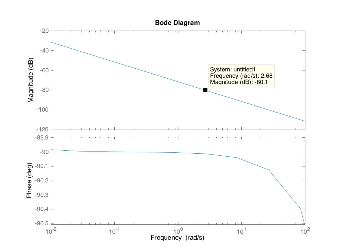
To move our bode plot up as to get omega_c = omega_n, desired = 1.8, we need to multiply our controller gain by K = 10^4 and adjust our phi to maintain the desired steady-state error.
This gives us the overall controller D(s) = 12.7261/(s+0.0268) and the desired system response.
Results
Combining the plant and controller in a unity feedback configuration, we get the following block diagram:

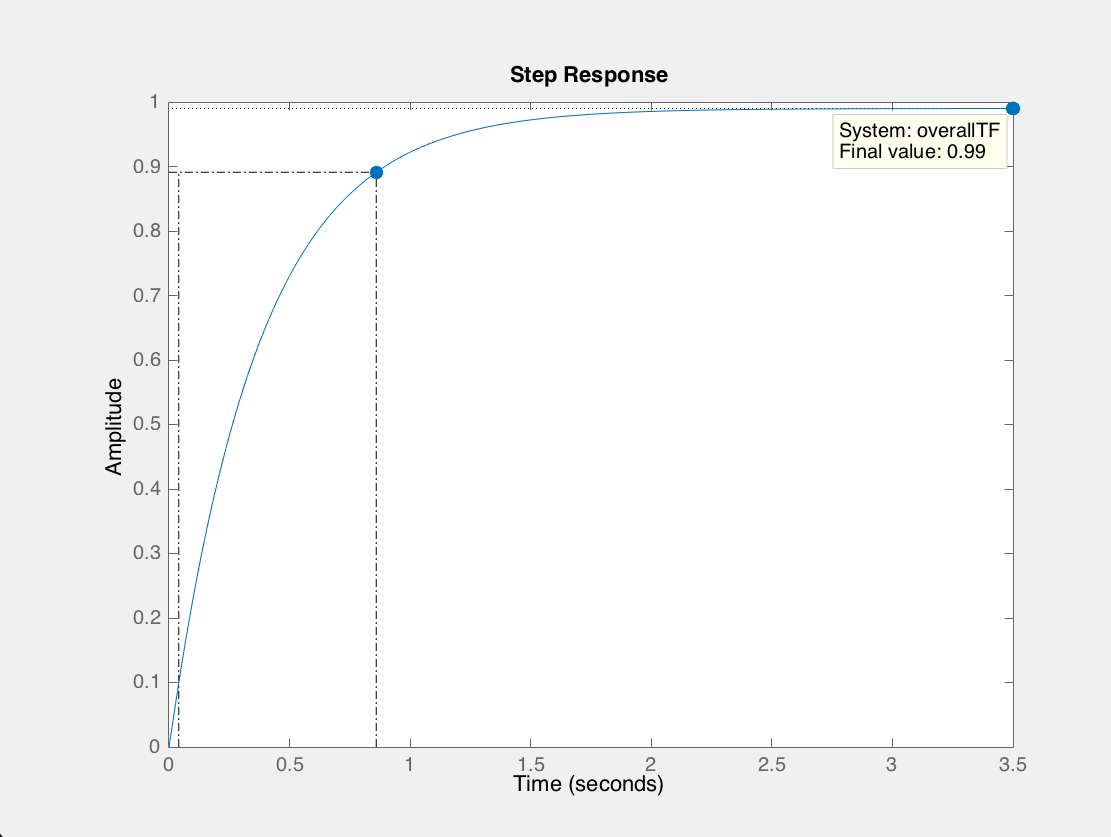
Which gives the resulting response to a step input of 5 m/s:
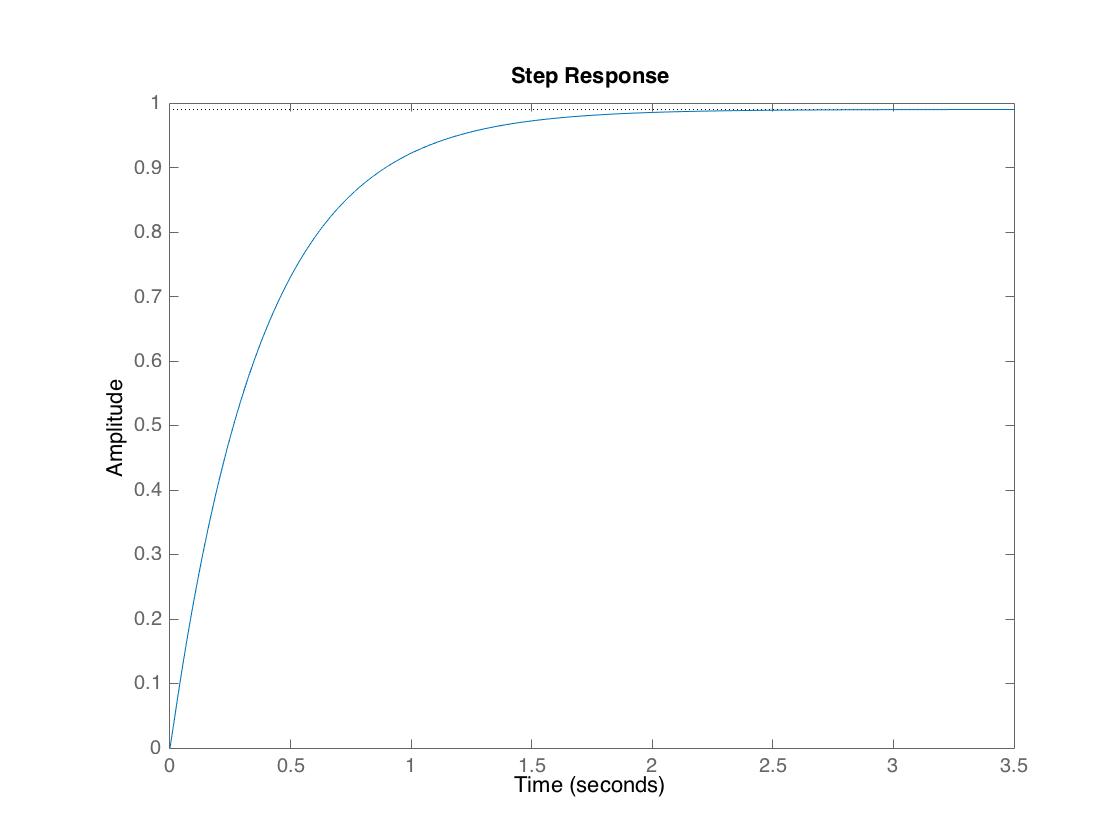
The response to a unit step with given rise time is:
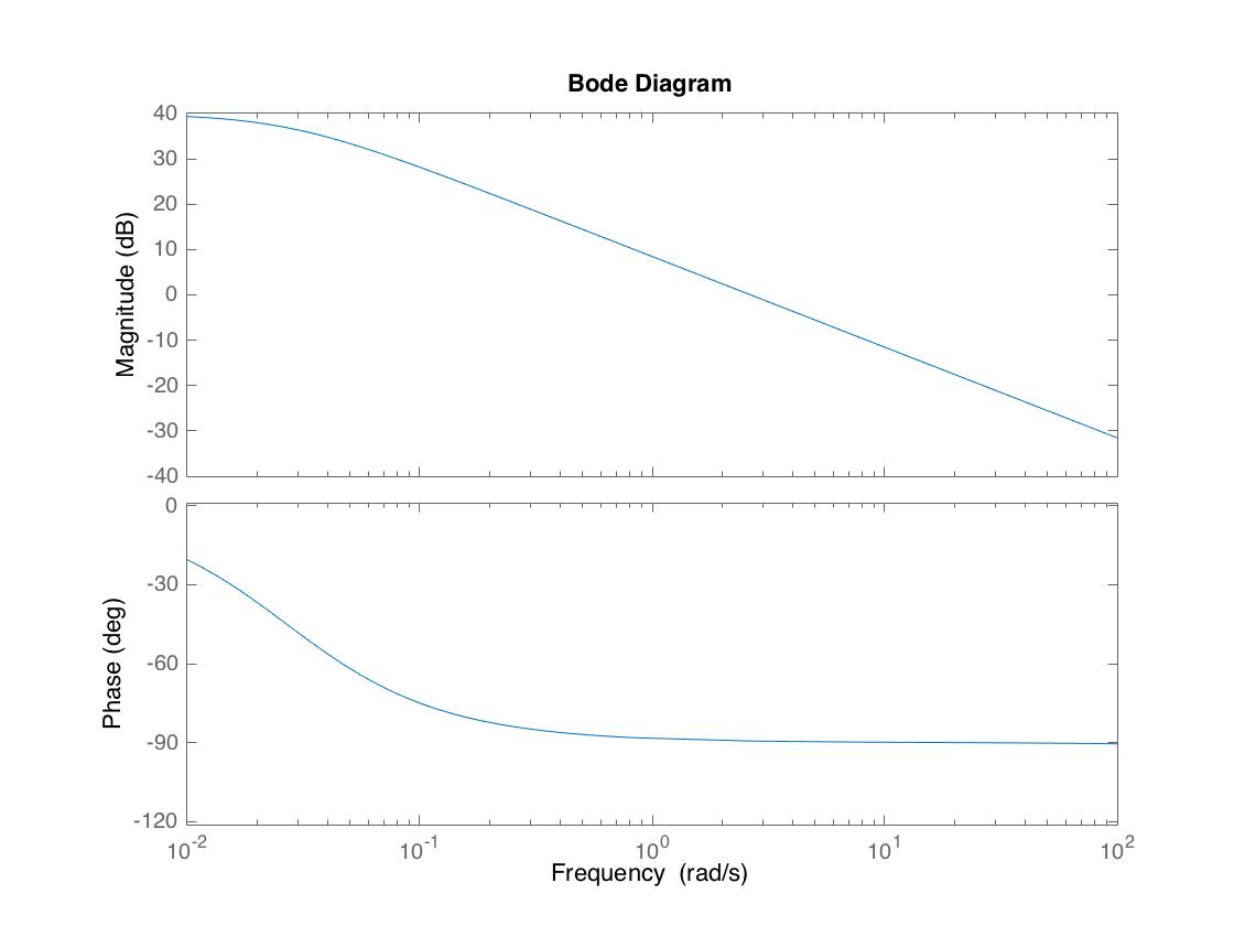
Additionally, the resulting Bode plot is:
Finally, if we are to put our system into a microprocessor, we would like to take time delay into account. From class we saw that time delay can be modeled as a block in the block diagram in the forward path. This block as the transfer function e^(-Td*s). The math behind this, however, can be complicated. As such, we may use the Pade approximation e^(-Td*s) = (1-Td*s/2)/(1+Td*s/2). Assuming a time delay of 1ms we add a time delay block to our overall block diagram. With this, we get the following diagram in Simulink:
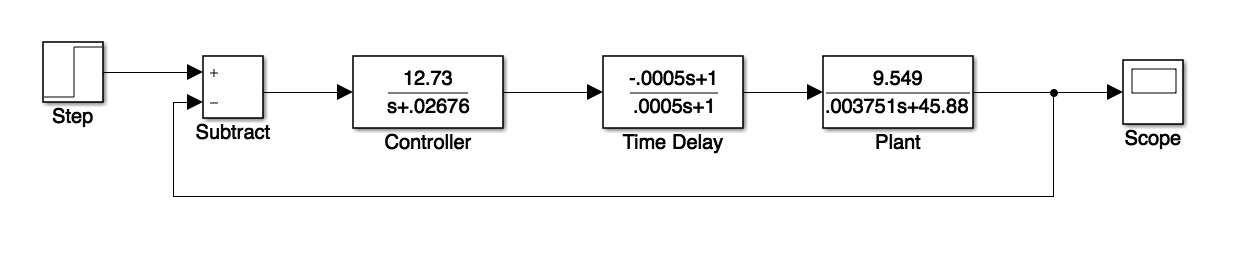
Which does not change change the overall system response in any noticeable way. This can be seen in the overall feedback system response of this block diagram:
Conclusions
Overall, the control exploration was successful. We began with discovering that the DC motor has pretty unreliable behavior in the open loop case. By using a simple controller of the form K/(s+phi) we were able to not only reduce the steady-state error to less than 1%, but also make the system have a rise time that would be both beneficial to power supply as well as fast enough to do quick robot scoring of poker chips. The controller was simple enough as to have enough variables to control 2 parameters, did not have a zero to make the system more complex, and had a single pole to make the system second order. Moving forward, we would want to do a few things. First, we would like to look at system response considering chip trajectory, possibly including air resistance and kinematic equations. Second, we would like to model our system in a more realistic way. A huge source or load torque comes from the chip running under our flywheel. This is not something we modeled and are not sure as to how we would do it. We might consider making it an impulse disturbance, but this might not give our system time to response. Modeling this in some way would make our system much more accurate. Regardless, this project gave us practice in using control parameters to produce a flywheel tangential velocity response that matches the desired specifications that we placed on it.
Acknowledgments
We would like to acknowledge our sister group, Katie Torigoe and Jesus Loza, for always being there to help. Additionally, we would like to thank the entire teaching team for making our controls experience so interesting and useful.
Files
- File 1: Attach:Flywheel_video.mov
- File 2: Attach:SSJ_MatlabSourceCode.docx Δ
References
As noted above, some of our system constants were found using the following websites:
DC Motor: pololu.com/product/2271