

Samuel Frishman John Alsterda

Cruise Control
Welcome to our project page for Stanford University's ENGR 105: Feedback Control Design class. Our goal is to design and analyze a control system using the tools we have learned this quarter.
Abstract
A cruise control system was designed and implemented on a small DC motor. We were interested in this topic because cruise control is a classic example in controls and is a system we encounter regularly driving our own cars. Additionally, as vehicles continue to be augmented with increasingly more automated features, the demand for engineers with experience applying these ideas will (hopefully) grow. Our goals were to write a controller using what we learned in ENGR 105, then to implement it on a physical system, and finally to reflect on the differences between what we expected from the mathematics and what we observed and on the physical motor.
Advanced Features: Implementation on a Physical System and Digitization.
Introduction
The chance to apply what we learned in class to a real physical system drove our motivation for this project. Plots and graphs derived from pure mathematics are useful tools to understand our world, but building a demonstration that users can interact with is equally important to develop intuition and trust in the theory.
Motor speed control is an ideal system on which to implement our theory, as the second order system is both interesting mathematically and simple enough that we were be able to get the controller working on a real motor with too much drama.
Plant Model
Our plant is an Igarashi DC motor driving a roller-skate flywheel attached to the motor shaft. The system dynamics include the electro-mechanical dynamics of the motor, as well as the mechanical dynamics of the flywheel. The plant's input is the motor drive voltage; its output is the angular velocity of the flywheel. A sketch of our model with relevant constants is below:

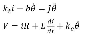
In order to control this motor over time with an appropriate voltage, equations were developed to describe its dynamics. We began by writing the time-domain equations for the system:

We then solved for the Laplace-domain plant transfer function:

The system can finally be represented in an open-loop block diagram:

A more detailed derivation of our model is shown below:

In order to solve for realistic voltages and motor speeds, our system parameters must be estimated:
- Resistance of the motor, R = 17.5 ohm (measured with multi-meter)
- Inductance of the motor, L = .0084 mH (measured time constant with oscilloscope and function generator; 𝜏 = L/R).
- Viscous damping of the motor, b = 0.0002 J/(rad/sec) (typical value for this size motor)
- Mass of the fly wheel, m = 0.17 kg (measured)
- Radius of the flywheel, r = .03 m (measured)
- Motor constant, Ke = .5 V/(rad/sec) = Kt = .5 Nm/A (motor datasheet)

Using the values above, we simulated the open loop plant in MATLAB. The input was a step function of 1 Volt; the output was the motor's angular velocity. The figure below shows the open-loop step response of our system. As expected, a step voltage input induced the motor's angular velocity to rise and then settled at a steady state final value.
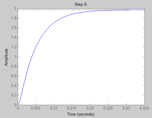
For practical application, this behavior is not quite acceptable. The speed appears to approach steady state smoothly, but this is not good enough. There are no means to control rise time, settling time, potential overshoots, and the impact of disturbances on the system. Furthermore, our physical plant and will surely deviate from this ideal mathematical description. Therefore, this open loop system must be closed with a feedback loop.
Control Design
To control the motor speed, we implement a PI (proportional and integral) controller and close the loop around the controller and plant described above. We predict this will be appropriate to eliminate error in this Type 0 system.


Now that our controller has a structure, its parameters must be given values. Defining of these values required a little thought because the methods we learned to tune PI controllers in class considered adjusting only a single parameter. This time we have two: Kp and Ki.
By first focusing our attention to the controller's initial response at time zero, we isolated Kp. This is possible because the integral correction weighted by Ki requires some time to build up and is therefore initially absent from the response. At time zero, the initial value theorem confirms applied voltage depends only on Kp:

Our constraint is that we do not want the controller to demand more effort than our physical system can provide. In this case, physical effort is our battery voltage of 15.3 V, and we will try to achieve 60 RPM or 2π rad/sec.

This is great progress! Next, to analyze the root locus, we factor Kp out of our controller:

We assessed the root locus for several Ki/Kp ratios and settled on Ki/Kp = 100. Here, we found that Kp values well under 2.44 still yielded very stable systems. That is, their roots were left of the imaginary axis with generous margin. As depicted in the root locus below, we set Kp = 1 and Ki = 100.

To confirm the stability of this root locus design, we consider the open loop Bode plots.

Here we find that our closed loop system has a Phase Margin of ~93 degrees and an infinite Gain Margin - decently far from instability. We hope any differences between our physical and ideal plants do not erase these margins.
As a final check, we plot our control effort and the system response over time to a step input of 60 RPM or or 2π rad/sec. We verify the effort won't exceed 15.3 V, and that the output settles to 60 RPM within a reasonable amount of time without a fantastic overshoot.


We were happy with the plots above. Let's see if we get it up and running on a physical system!
Results
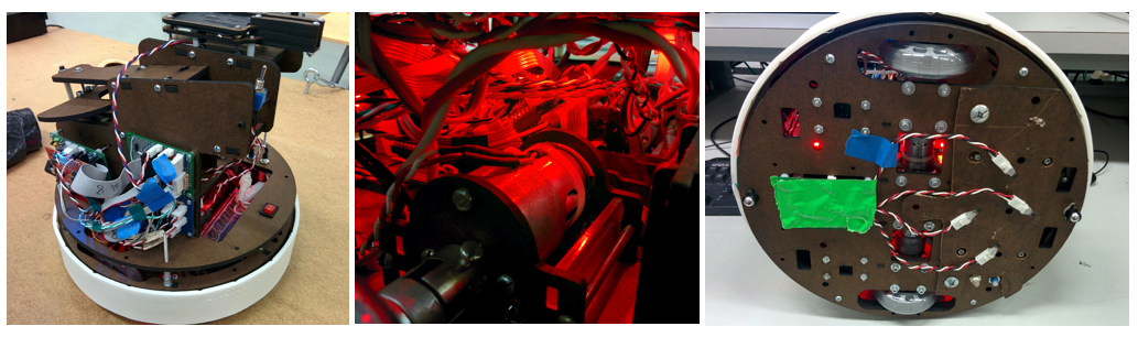
To bring our theoretical model to the real world, we wrote our controller into Marco Robotio, one of this quarter's ME 218 robots. The C code module containing this controller is attached at the end of this report. Our test motor can be seen in the center shot below. On right, the bot has been placed on its side so we could perform our measurements.
Our first results were disappointing and puzzling. We set our experiment to track a reference input of 60 RPM. As shown below, our proposed gains caused the physical output RPM to oscillate wildly!
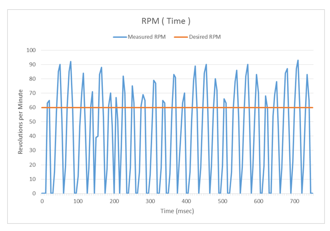
Extreme undershoot and overshoot were measured as the controller attempts to find 60 RPM.
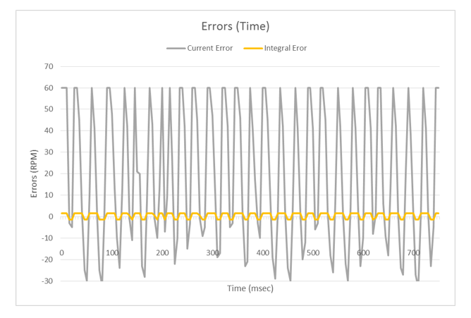
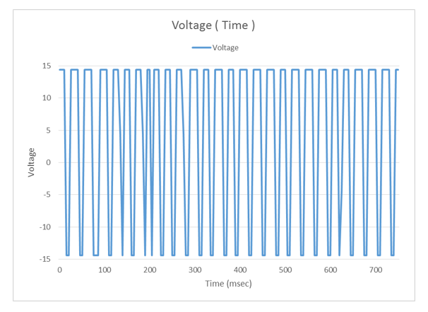
The battery voltage is consistently railed as the small integral error accumulated above is amplified by 100 times.
We believe our error may be the result of one or more of the following sources:
- Our system transfer function is missing a pole that draws the root locus into the right half plane
- Some physical constant measurements may be incorrect
- Digitization of this continuous system injected instability
- Our battery voltage could not follow the controller's desired effort
Our class briefly introduced the concept of using the Z-Domain to probe digitization effects. Let's see if we can apply it to glean any evidence of instability. The closed loop system was digitized by use of "Tustin's Method" with a sample rate of 5 msec.

"Feedback Control of Dynamic Systems 7th Edition," states that z domain poles must have magnitude less than 1 to find stability. A pole lies on the real axis at 1 above, possibly indicating a source of our physical motor's disagreement with the continuous mathematics.
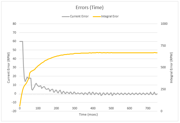
Moving forward, we found that setting Kp = 1 and reducing Ki to .1 yielded fantastic results:


We even found the system to be stable in response a roughly Type 0 disturbance, a finger providing friction to the flywheel for a few seconds:


Before we get too comfortable with these gains, let's go back and make sure they satisfy the continuous mathematical model. First, the root locus shows confirms we aught to be stable, albeit with a much closer pole to the right half plane.

Next, the open loop Bode plot similarly confirms stability:
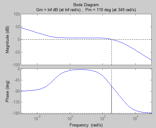
In summary of our results, setting Kp = 1 and Ki = .1 worked both mathematically and in the real world.
Conclusions
Most importantly, we learned that physically implementing a mathematical model is not easy and can produce many unexpected results before (or if ever!) yielding satisfactory outputs. Luckily, we were able to stabilize our system. Overall, we think our plant model and control scheme worked well to control the RPM of the flywheel. However, questions certainly remain regarding why pushing the Ki gain made the system oscillate and become unstable. Future work would focus on answering this question by pursuing the possible error sources listed above in the Results section.
Files
Code and Simulink models should be linked here. You can upload these using the Attach command.
- MATLAB code for simulations Attach:frishman_alsterda_project.zip
- C Code for running the motor Attach:frishman_alsterda_SpeedControl.zip