

Sanjay Srinivas Davy Lu

A launch of a rocket carrying
a GPS satellite as a payload .
Controlling velocity of a rocket-launched satellite
Project team member(s): Davy Lu, Sanjay Srinivas
Abstract
This project details a control system for a rocket-propelled satellite, where we control the satellite's final velocity as a function of the gravity-adjusted nominal lift force. In satellite applications, controlling final velocity at a desired settling time and with low overshoot is critical in order for the satellite to be properly in phase with the earth's rotation. We compare our analysis, which requires constant values of the rocket's mass and acceleration due to gravity, with a nonlinear system analysis using SIMULINK, which allows us to vary m and g with time. The ability to model changing mass is especially important for a satellite, where rocket fuel comprises a large percentage of the system's initial mass. Our final control system was a proportional-integral-derivative (PID) controller with lag compensation, which allowed us to achieve a stable step response with a settling time of 886 seconds (close to our desired value of 900 seconds, typical for satellite launches) and maximum overshoot of 2.6 per cent. Conversely, the non-linear system with the same PID and lag compensator values was not able to converge to a desired steady-state velocity, suggesting that SISO control theory fails to account for variable coefficients.
Introduction
Low-earth orbit (LEO) satellites have applications extending from GPS to weather monitoring and satellite imaging. In many cases, it is crucially important that these satellites be geosynchronous, meaning that they need to match the Earth's rotational speed. This need for controlling the satellite's final position and velocity led us to thinking about using a controller to stabilize the satellite's behavior. We also wanted to analyze the usefulness and limitations of linear, single input - single output control theory by comparing our model to a more physically realistic system using SIMULINK.
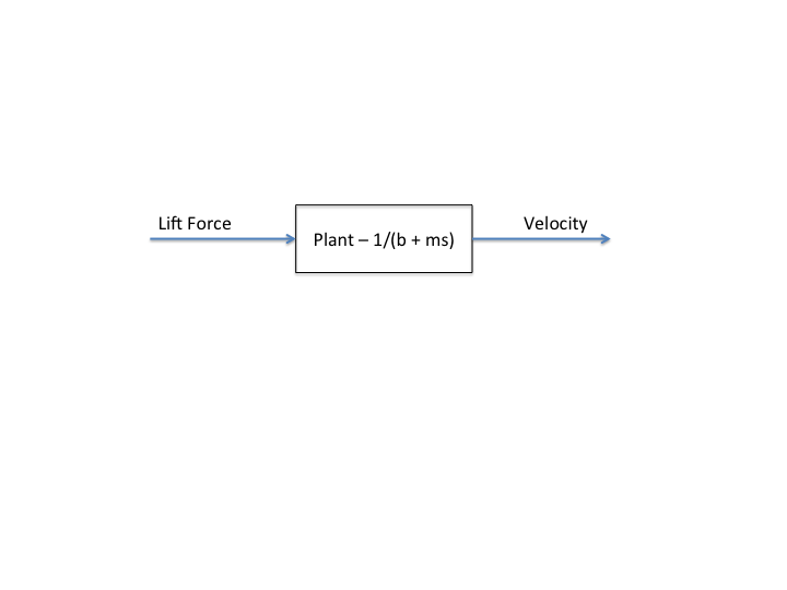
Plant Model
We use Newton's equations of motion to determine the controlled velocity of an accelerating rocket. We model drag due to air resistance as a linear damping force proportional to the rocket's velocity. In the linear case, we take the mass of the rocket, m, and acceleration due to gravity, g, as constant. Assuming no motion in the horizontal direction, this results in 3 forces acting on the rocket; lift, drag, and gravity. Because gravity exists as a "steady-state" force that is not dependent on the rocket's velocity, we define F 'lift = Flift - mg, which simplifies the control analysis, allowing for a closed-form solution to the plant transfer function.
Using Newton's Second Law, F=ma, we determine the equation of motion for the system:
Flift - mg - bv(t) = mv'(t)
Simplifying the equation with the nominal definition of lift force established earlier in the section, and computing the Laplace transform of the equation:
F 'lift = bV(s) + msV(s)
Factoring the left side, we can find the system's open-loop transfer function V/F 'lift:
V/F 'lift = 1/(b + ms)
The open-loop block diagram of the system is shown below:
Below is the derivation of the open-loop transfer function from the system's equation of motion.

Our list of parameters includes:
m: initial mass of the rocket - using the Saturn V rocket, we estimate m = 500,000 kg
b: Linear damping coefficient used to calculate drag force. Sixty-nine seconds into the Saturn V launch, the rocket experienced maximum dynamic pressure, in which it underwent approximately 2.046 * 106 Newtons of drag force as it was moving at roughly 1000 m/s. Using a linear model for drag, we compute b = 2046 N*s / m.
Using the constants defined above, and the open-loop transfer function mapping lift force (the input) to rocket velocity (the output), we modeled the system's open-loop behavior to a unit step input of 1N, which we observed over 2000 seconds.
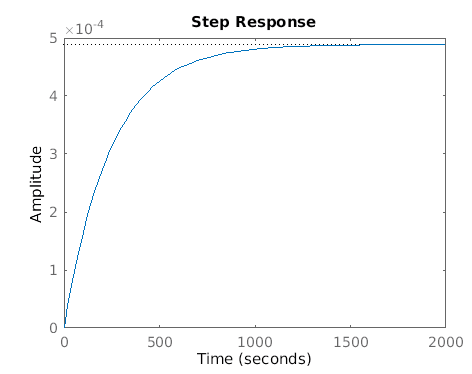
Although the open-loop behavior converges to a final steady-state value, it does not converge in a suitable time-scale (reaching a steady-state value well after the desired 900s) and has substantial steady-state error. We need to design a controller that drives steady-state error close to zero while increasing the speed of response. We also hope to replicate, or at least approach, the lack of overshoot in the open-loop system.
Control Design
We used a proportional-integral-derivative (PID) controller with low integral gains to decrease overshoot while still driving steady-state error to 0. To speed the response up to the desired settling time, we added a lag compensator with a negative zero and pole, as adding a negative zero to the system increases its response time, getting us to steady-state earlier. To compensate for the large mass of the system, we set the proportional and derivative gains relatively high, allowing us to stabilize the system in a reasonable time-scale.
We let our PID controller G(s) = kp + kd*s + ki/s, where kp, kd, and ki represent the proportional, derivative and integral gains, respectively. Our lag compensator L(s) = (s+z)/(s+p), where z and p represent open-loop zeros and poles, and z>p. We let kp = 500, kd = 500, ki = 3, z = 45, and p=10.
The closed-loop block diagram, including the controller and lag compensator, of the system is shown below:

For our Simulink model of the variable-coefficient system, we created a block diagram that showcases an additional feedback loop that integrates the velocity output of our previous design to acquire position and applies the equations of gravitational pull to this new input to get a constantly changing G. To arrive at an equation for a linearly-decreasing mass, we started with the form:
m(t) = a +bt
L[m(t)] = M(s) = a + b/s^2
M(s) = (as^2 + b)/s^2
The variable a would be our initial mass, which was already stated to be 500,000 kg. The variable b was chosen by taking the difference of the intial and final masses of the Saturn V rocket at each stage of its launch and dividing by the total time it took to reach its final mass. Thus our final equation was:
M(s) = (500000s^2 - 3028)/s^2
This combined with our now-changing gravity term would provide a good basis of comparison for our assumptions of keeping them constant, as graphing both could easily tell us how big the error of assuming a linear system could be.
Block Diagram of Non-linear System

In order to determine the values of our controller gains, we first found the range of kp, kd, and ki that would stabilize the system using a Routh array on the characteristic equation 1 + DG.
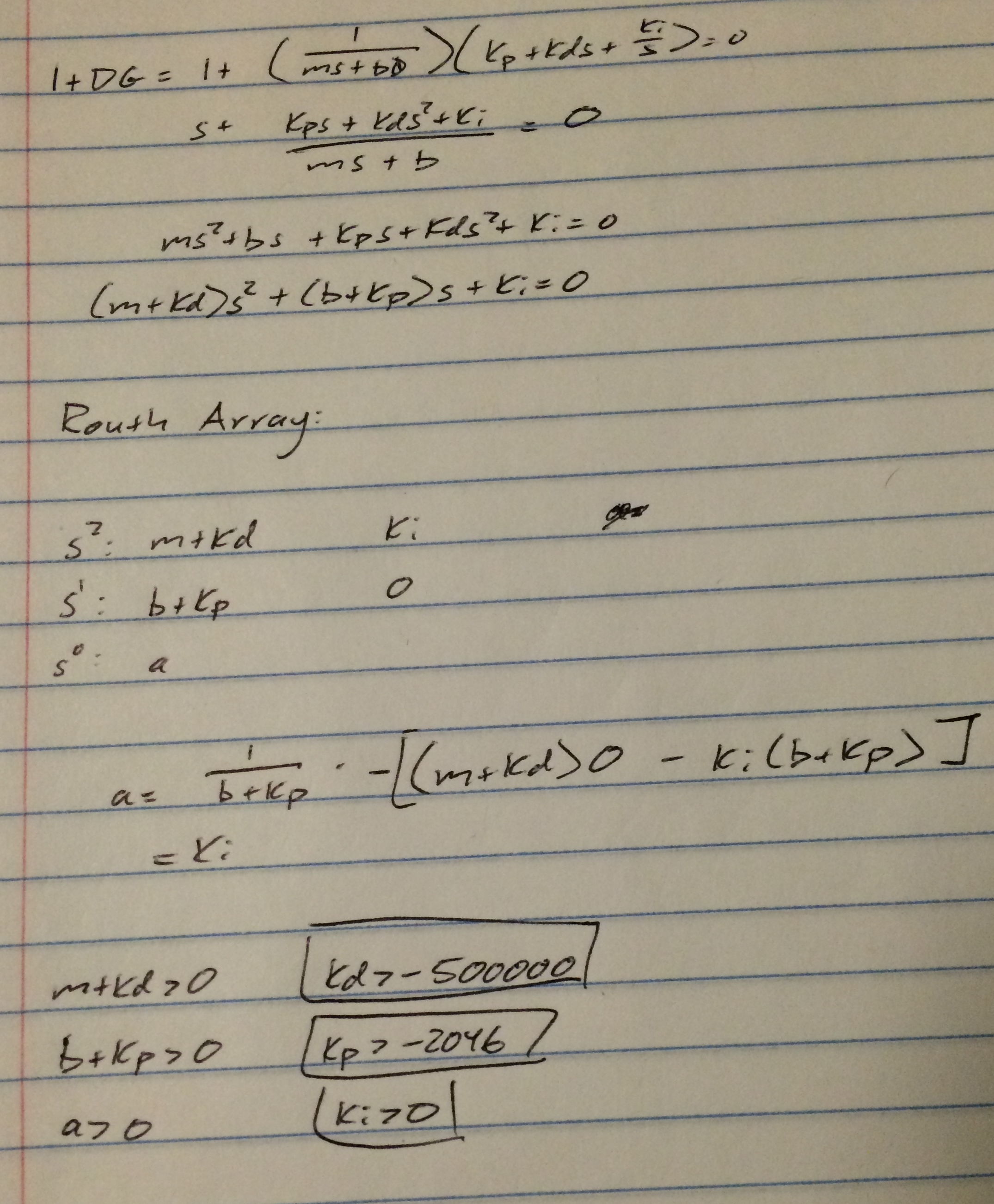
The Routh array shows that any positive controller gain will stabilize the system. We confirmed this by graphing the root locus for the open-loop system.

Since we did not have to worry about stability, we instead selected parameters according to how they would achieve our other design specifications: a settling time of 900 seconds and low overshoot.
We were originally interested in designing a PD controller because it would be a relatively simple controller that would result in stability with no overshoot. We modeled a system with low proportional gain (kp = 3) and high derivative gain (kd = 300) and found that there was unacceptable steady-state error, despite eventually stabilizing with low overshoot. Additionally, the response time was slow due to low kp; this controller too closely resembled the open-loop behavior.

To fix the steady-error, we introduced integral control. We increased the value of kp and kd to 500 to speed up the response and try to minimize error. To maintain our original goal of little to no overshoot, we left the value of ki low (ki = 3). This controller converged to a steady-state value of 1, but was again too slow, and we did not want to keep increasing the value of kp to speed up the response (as this would eventually become hard to physically realize with a real controller).

Instead, we implemented a lag compensator to speed up the response. To speed up our response time, we knew that the negative zero we added with our lag compensator needed to be substantially greater in magnitude than our pole. As our Routh Array shows, the system will be stable for all values of k, but we were working with time constraints based off of real-life values we found online. As a result, we settled on a a zero of -45 and a pole of -10, as this left our system in steady-state around 900 seconds, which satisfies our design specifications. This way, we could keep our PID gain realistically low.
Results
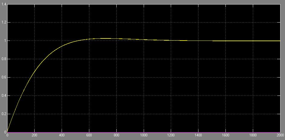
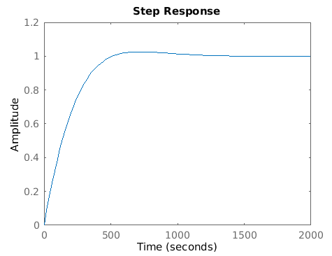
This is our closed-loop, second-order, linear system with the assumed constant mass and constant G. It matches our step input from our Matlab plotting. The input is a unit step with a end time of 2000 seconds. We drove steady-state error to zero with a settling time 886 seconds. The input represents the nominal lift force of the rocket, while the output is a desired velocity.
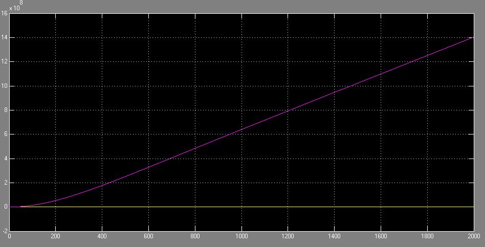
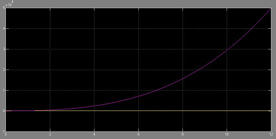
This is the closed-loop, second-order, non-linear system with variable coefficients - namely a linearly decreasing mass and a G that decreases as the rocket gains altitude. The input is a step of 1+(rocket initial mass * 9.8). Since the variable mass and G is being fed back, we expect this graph to be accurate to our linear assumption for a very short period of time, as we are starting with an equivalent step input. Then, as time as well as the difference between the assumed mass / gravity and actual mass / gravity starts increasing, the non-linear system starts diverging from our original graph.
Conclusions
Our experiment highlighted the drawbacks of doing linear systems control. We initially started with the idea of a rocket with a constantly decreasing mass and tried to apply the lessons learned in this class to design a controller for it. We quickly found out that we were breaking a fundamental assumption about the limitations of the type of controls we have learned, as our model had variable coefficients. Instead, we decided to use Simulink for the nonlinear control and assume for our system that mass and gravity was constant. By applying a step input to both of these on the same graph, we clearly saw the degree of accuracy our assumption had. Assuming constant mass and gravity was accurate for less than ten seconds. We saw the Simulink non-linear control take off and overshoot our graph, which makes sense, as a lower mass and gravitational force would mean a higher velocity, and within ten seconds, a lot of mass in the form of expended fuel would have already been lost. The system response we achieved was not accurate but very satisfactory in the context of comparing the difference between linear and non-linear control. In the future, we would play around with different burn rates of rockets, and therefore the rates that mass decreases, as these figures are readily available online. For instance, it would be interesting to see how tricky velocity control for a rocket gets when the burn rate is a negative logistic curve. Another thing to look at would be to factor in how drag is constantly changing due to velocity as well, as it is not a constant damping force in real life.
Acknowledgments
We would like to thank Adam Leeper for helping us refine the focus of our project, especially in emphasizing the differences between the linear and non-linear systems. We would also like to thank Allison Okamura for doing a wonderful job teaching this class.
Files
Code and Simulink models should be linked here. You can upload these using the Attach command.
MATLAB Code for open-loop system
clear all
close all
clc
m = 5*10^5;
b = 2046;
s = tf('s');
sys = 1/(b+m*s);
step(sys,2000)
MATLAB Code for final closed-loop system
clear all
close all
clc
m = 5*10^5;
b = 2046;
kp = 500;
kd = 500;
ki = 3;
s = tf('s');
D = 1/(b+m*s);
G = kp + kd*s + ki/s;
L = (s+45)/(s+10);
sys = (D*G*L)/(1 + D*G*L);
step(sys,2000)
stepinfo(sys)