Re-entry Vehicle Control Design

Project team members: Walter Maier, Jonathon Schut

Abstract

Given a growing interest in space travel by both private enterprises and the general public, there is an increased need for creating reliable re-entry vehicles to return humans and equipment safely to a planet's surface. Therefore, in an attempt to better understand the design of re-entry vehicles, we have constructed a simplified model of the dynamics surrounding a vehicle's descent that includes an integrated controls system for regulating the re-entry process. For modeling this system, the plant incorporates the effects of the major forces acting on a capsule during the supersonic retro-propulsion stage of re-entry, including: atmospheric drag, gravitational attraction, and rocket thrust. Since safety and reliability are key requirements for a re-entry vehicle, the goal of the control design is to obtain a quick descent time and reach a steady state altitude of 3-5 km. The fast descent will minimize the heating caused by aerodynamic drag, thereby decreasing the necessary mass of the heat shield, and the steady altitude will allow for a safe deployment of a parachute to safely carry the capsule to the surface. Ultimately, we have designed a PID controller that guides the capsule's descent to the desired/stable altitude range in under 2 minutes without raising any serious safety concerns about surface impact.

[Due 3/2, 3/4, 3/7, 3/11:] Give an increasingly polished one-paragraph description/summary of the project, which includes information like the motivation for considering the particular plant you chose, the control design goal, and the resulting implementation and results. More information can be added as the project progresses.

[Due 3/2:] Advanced Feature - this control design project will incorporate the following feature for increased complexity:

1. A Simulink model of the nonlinear re-entry control system.

Introduction

[Due 3/2:] Entry vehicles represent a back bone of space exploration. They have delivered probes to the surface of Mars and have returned humans back home to Earth. Most recently, astronaut Scott Kelly returned to Earth on a Soyuz re-entry vehicle. To continue pushing humans further into outer space, new entry capsules will need to be utilized. Unlike Earth, other planets have extremely thin atmospheres, making deceleration and heat dissipation more difficult. This problem can be realized from the most recent Mars missions. The effects of thin atmospheres will be amplified as humans begin to visit Mars and send probes farther away from Earth. The new capsules designed will require new and more advanced control systems to complete their mission with the greatest margin for success.

Developing these future re-entry systems requires innovative technologies such as supersonic retro-propulsion (SRP), which "involves initiating propulsive deceleration at supersonic Mach numbers by directing engine thrust into the oncoming freestream flow."[1] By firing the rocket thrusters, the vehicle experiences two forms of drag that are characterized by the following coefficients:
* Aerodynamic drag coefficient for drag D: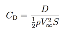

* Propulsive drag coefficient for thrust T:

These drag forces, coupled with the gravitational force of the central body, constitute the basic dynamics of the supersonic retro-propulsion stage of the vehicle's re-entry. Given the complexities associated with accurately modeling the density of a planet's atmosphere, we have assumed that this additional parameter in the drag coefficient equations is constant. The equations of motion can then be derived from this simplified model of the forces acting on a re-entry capsule.

Plant Model

[Due 3/4:] Describe your plant model.

1. Description of the Model:
In our model, a capsule (mass m) equipped with retro-propulsion rockets is descending into a planet's atmosphere at supersonic speeds with a particular angle of attack. The model incorporates the three major forces acting on this re-entry vehicle, including: atmospheric drag, gravitational attraction, and rocket thrust. The following is a force-balance diagram that outlines our simplified model of the physical system:

2. Time-Domain Equation of Motion:
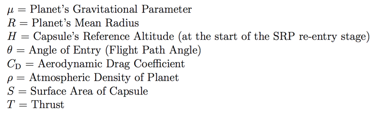
Since we are interested in controlling the vehicle's descent, we are considering the motion of the capsule in the direction it is traveling, as shown by the unit vector x in the diagram above. Therefore, after analyzing the diagram of the forces acting on a capsule, we derived the following equation of motion (assuming a constant angle of entry):

where the parameters in the equation are:

3. Block Diagram of the Open-Loop System:
Although we cannot derive a Laplace-domain transfer function for our model due to nonlinearities, the following is the open-loop block diagram with thrust T as the input, and the distance traveled x as the output:

where the equation for the x - double dot block is

4. Derivation of the Model:
To derive the time-domain equation of motion listed above, we adopted a reference frame fixed to the capsule's direction of motion such that a single quantity x could describe the vehicle's descent. In doing so, the component of the gravitational acceleration in the x-direction is positive, with the drag and thrust opposing this motion. The gravitational acceleration is computed using Newton's formulation due to the high altitude of the capsule during re-entry. Also, since the thrust of the retro-propulsion is effectively an input for our system that we can control, we decided to define it as an individual force (T) separate from the aerodynamic drag. Accounting for all of these factors, the derivation is as follows:

5. List of Parameters for the Model:
In order to have actual values for the parameters in the equation of motion, we are simulating the re-entry of an Apollo capsule into Mars' thin atmosphere at a relatively small angle of attack:

• Mass of the Entry Capsule = 7000 kg (including mass of propellant - assumed constant)
• Drag Coefficient = 1.4
• Radius of Mars = 3396.2 km
• Initial Atmosphere Height = 25 km
• Surface Area of Capsule = 0.000011946 km^2
• Gravitational Parameter of Mars = 42828 km^3/s^2
• Flight Path Angle = 5 degrees = .0873 radians
• Atmosphere Density of Mars = 20000000 kg/km^3
• Initial Atmospheric Entry Velocity = 4 km/s

- Note: These values are based off of the results found in literature [2][3], with the initial reference altitude and velocity of the capsule being approximated from typical re-entry scenarios [4].

6. Simulation of the Open-Loop Behavior of the Plant:

To simulate the open-loop behavior of our plant, we assumed that the retro-propulsion thrust is a step input of a certain kilo-newton magnitude into our system (100 kN). The following is a plot generated by MATLAB based off the results of our Simulink model that illustrates the altitude (H - x*sin(theta)) of the capsule over the duration of the thruster burn:

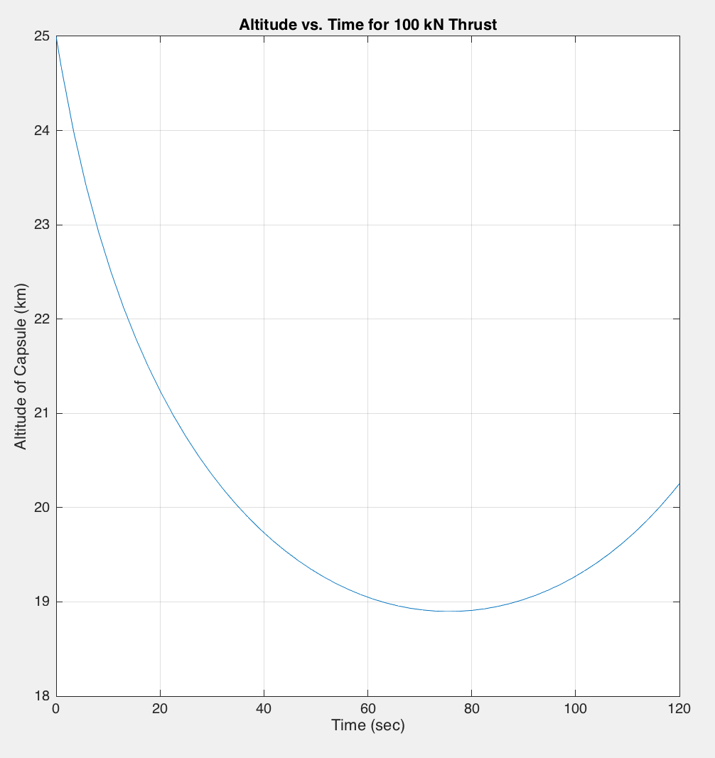
Thus, we observe that engaging a constant retro-propulsion over the course of 70 to 80 seconds can effectively slow the capsule's descent to a halt such that a more manageable landing could be obtained. The undesirable aspect of the open-loop behavior is the instability inherent with providing a constant thrust. As illustrated in the plot above, supplying a constant retro-thrust beyond 80 seconds results in the capsule gaining altitude and eventually exiting Mars' atmosphere, which is counter-productive for our system. Also, the point of closest approach to Mars' surface is approximately 19 km, which is not optimal for the purpose of re-entry. Thus, we would like to be able to control how this thrust is applied in order to have the capsule's trajectory converge to a more desirable path of descent that brings the capsule closer to Mars' surface during approach.

* First, describe the model in words. * Second, give the time-domain equation of motion for the model and (if possible) the Laplace-domain transfer function for the model. * Third, show a block diagram of the open-loop system. * Fourth, show the derivation of your model as inline equations, as inline images, or in an attached file. * Fifth, give a list of parameters of your model, what values you are using for those parameters, and how you found/estimated them. * Sixth, provide the results of a simulation or experiment that shows the open-loop behavior of the plant. Clearly describe the input and output signals. Explain what is not acceptable about the open-loop behavior.

Expected length: Approximately 1-2 "pages" if this were on 8.5" x 11" paper.

Control Design

1. The Control Approach:

Based on the open-loop results for our system, we want a controller that provides a stable closed-loop response in which the capsule converges to a desirable altitude in an optimal amount of time to avoid heating issues. Thus, since we need a reasonable response time with reduced steady-state error, we have implemented a PID controller to incorporate the time-response effects of zeros and poles. For instance, with derivative control, we can decrease the settling time and overshoot of the output signal such that the capsule's descent avoids the danger of a fatal collision with the surface and converges more quickly to the desired altitude. Also, with the combination of integral and proportional control, we can decrease the steady-state error of the system to yield an improved re-entry trajectory that is more accurate in attaining the desired altitude. The specific goal behind implementing this PID controller in our system is to design/tune its various gain parameters until the resulting response of the closed-loop system fulfills the requirement of achieving a stable altitude around 3-5 km in about 2 minutes or less from the start of re-entry at 25 km.

2. An Appropriate Mathematical Description of the Controller:

With a PID controller being a combination of proportional, derivative, and integral control, it has the following form:

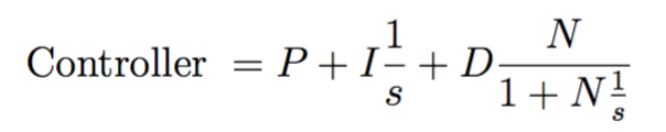
where the variable N is a filter coefficient that is added to act as a fast pole in order for the derivative controller to be physically realizable. This filter coefficient, and the gains P, I and D are tuned in order to attain the desired response to a reference step input.

3. A Detailed Block Diagram of the Closed-Loop System:

For the closed-loop system, we are using a unity feedback loop with the PID controller computing the necessary thrust based on the error between the desired x and the output x. This is illustrated in the following Simulink block diagram:

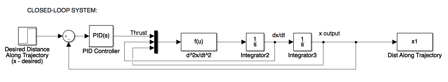
where the function f(u) is the same as before, and the PID controller has the format given above, with:

• Proportional (P) = -2634.3668
• Integral (I) = -73.8171
• Derivative (D) = -12728.396
• Filter Coefficient (N) = 207.8378

Note that the various gain terms of the controller are negative due to the set-up of our system, in which the equation of motion has the thrust T being subtracted from the acceleration. Thus, in order to account for this subtraction, the controller is effectively negating the control effort for the closed-loop system. In addition, the input to the model is a step value of the desired distance along the trajectory (x_des). This value is calculated using the convergence altitude (H_des) and the following trigonometric identity:

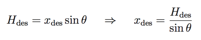
so for a desired altitude of 5 km and a 5 degree angle of attack, we have

for the desired distance along the trajectory.

4. Derivation of the Controller Parameters:

Since our system is inherently non-linear due to the presence of aerodynamic drag, we are not able to apply the controller design techniques that we learned about in lecture. Instead, we have taken advantage of MATLAB/Simulink's ability to linearize the plant and provide a "PID Tuner." This PID tuner includes a step plot for reference tracking in which the gain/coefficient parameters can be updated according to user preferences concerning the speed and transient behavior of the response signal. Attached below is a pdf file that describes our method of manually tuning the gain/coefficient parameters for the PID controller until a desirable response was attained. Ultimately, the refined PID controller that satisfies our system control goals has the following parameters:

• P = -2634.3668
• I = -73.8171
• D = -12728.396
• N = 207.8378

The plot of the altitude versus time for this final design of the controller is given below in the "Results" section.

This file contains the full outline of the iterative design of our PID controller: Attach:MS_ControllerDesign.pdf

[Due 3/7:] Give your control design approach. * First, describe the control approach in words. * Second, give an appropriate mathematical description of your controller. * Third, show a detailed block diagram of the closed-loop system, with signals and blocks clearly labeled. * Fourth, explain the derivation of your controller parameters and (if appropriate) the evolution of your controller through the design process. Include information as inline equations, as inline images, or in an attached file.

Expected length: Approximately 1-2 "pages" if this were on 8.5" x 11" paper.

Results

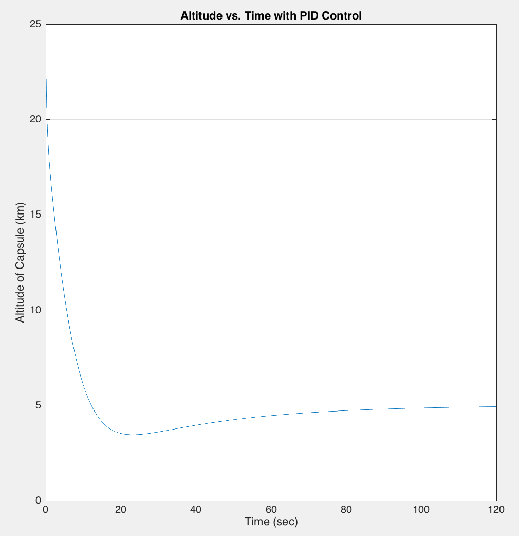
Clearly, the graphical results from our Simulink model illustrate the capsule reaching a steady state altitude of 5 km at about 110 seconds after beginning re-entry at 25 km. Furthermore, the capsule reaches the desired 3-5 km altitude range in approximately 15 to 20 seconds, without dropping below 3 km during the entire descent. Concerning time specifications, the closed-loop system response has a rise time of approximately 10 seconds, a settling time of about 100 seconds, and a peak overshoot of about 7%. From this, the damping ratio was determined to be 0.6461. Increasing this damping would slightly reduce the overshoot, but this would also increase settling time and possibly introduce more steady-state error. Therefore, given this tradeoff between possibly dangerous overshoot and settling time, we opted for a closed-system/controller configuration that yielded acceptable results in terms of these parameters. The final time characteristics of the closed-loop system response correspond to achieving the desired/stable altitude range in under 2 minutes with an overshoot that is reasonably safe.

These results were obtained by inputting a step reference of 57.37 km, representing the distance the capsule needs to travel to reach an altitude of 5 km. The output is the distance travelled by the capsule, which we can use to plot its altitude (as shown in the plots above). Also, in order to attain the closed-loop response that satisfied our two control goals for altitude and descent time, we needed to implement a PID controller with the following parameters:

• Proportional (P) Gain = -2634.3668
• Integral (I) Gain = -73.8171
• Derivative (D) Gain = -12728.396
• Filter Coefficient (N) = 207.8378

Concerning the values of these gains, we observe that derivative control plays a major role in regulating the capsule's retro-propulsion during the descent. This seems reasonable because, in controlling the behavior of a re-entry trajectory, we would expect to place significant bias on possible future values of the error in order to adjust current control effort appropriately. However, since we are unable to build a physical control system, we do not know whether these magnitudes in the gains (especially the derivative gain) are actually feasible.

[Due 3/11:] Provide the results of simulations or experiments that clearly show the closed-loop system behavior. Clearly describe the input and output signals.

Expected length: Approximately 1 "page" if this were on 8.5" x 11" paper.

Conclusions

Overall, we believe that our system with an integrated PID controller is quite successful in its application of controlling the descent of a re-entry vehicle. Based on our final results, we achieved a desirable trajectory that placed the capsule at an altitude of 5 km while greatly reducing descent time. This is advantageous as the capsule will have less exposure to the adverse effects of aerodynamic heating. Unfortunately, we could not eliminate the "overshoot" of the re-entry below the desired 5 km, but the PID controller is capable of restricting the magnitude of this overshoot to within an acceptable/safe range. Future work would involve relaxing our assumptions in modeling the physics of re-entry. For instance, instead of a constant angle of attack, the flight path angle would become a function of the descent. Also, the assumptions regarding the atmospheric conditions would be relaxed, as density is a function of position and time. These additional dependencies would drastically affect the plant and the resulting system response. Finally, another goal would be making the system more realizable by reducing controller effort (thrust T) and adding a more accurate drag model.

The uncontrolled simulation reaches a minimum altitude of 19 km at 75 seconds. The controller effectively reduced the descent time by about 30 seconds and positioned the capsule at the desired altitude. This reduction in rise (descent) time means less aerodynamic heating experienced by the capsule. Thus, the controller can be considered a success. The controller does allow the capsule to undershoot 5 km, reaching 3 km. Due to the undershoot, a faster rise time cannot be achieved without pushing the capsule too close to the surface.

Files

The Simulink and MATLAB code for our project:

• The MATLAB code that implements the Simulink model and plots the output response: Attach:MS_Project.zip
• The Simulink model for our nonlinear system (includes both open-loop and closed-loop models): Attach:MS_ProjectSim.zip

References

1. Description of SRP for re-entry: "Development of Supersonic Retro-Propulsion for Future Mars Entry, Descent, and Landing Systems"
2. Parameters for the Apollo Capsule: "Apollo Command Module"
3. Parameters for Mars: Mars Fact Sheet
4. Example Entry Trajectories for Mars: "Aerothermodynamic Design of the MarsScience Laboratory Backshell and Parachute Cone"

! Wiki examples

Here is how to link to a file (note that you may need to compress/zip your code and CAD files into zip files so that that wiki %comment$will let you upload them, due to file type restrictions): Attach:HapkitTest.ino.zip

Here is how to add an image:

Here is how to link a youtube video: