The Little Car that Could

Michaël Dooley, Brian LaBlanc, Joshua Phelps, Enrico Vittori

Introduction

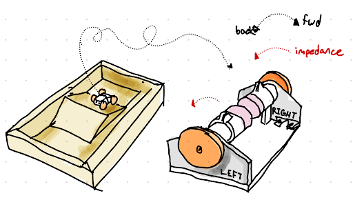
Figure 1. Ramp and controller sketch

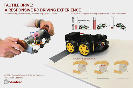
In this project, we wanted to create a basic remote controlled car that communicates environmental impedance back to the driver. The goal is that this car can communicate difficulty/ease while driving up/down hills, and let the user know when the car is “blocked” by an object or wall. We created our own velocity-based controller for the task, and communicated controls and impedance data over Wifi using ESP32s. All code can be found on Github.

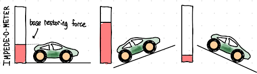
Figure 2. Motor impedance visualization

Background

Reflecting a remote vehicle's drive resistance back to the driver isn't a new idea, but it's a thin and scattered part of the haptics literature. Most “haptic driving” work/literature is about force-feedback steering wheels for racing sims, which isn't what we were after. We wanted bilateral teleoperation of a mobile robot, where the load the drive motors feel (hills, walls, rough terrain) shows up as resistance in the controls.

The closest published parallel to our project is Rösch, Schilling, and Roth (2002). They drove a differential-drive RC car over the network with a two-motor force-feedback joystick, computing the feedback force by fusing a front force sensor, wheel velocity, and drive motor current. Hitting an obstacle, climbing a hill, or slipping on a slick surface all came back to the operator's hand. That's basically the system we set out to build, minus the current sensing we wish we'd had. The other directly relevant work is “haptic tele-driving with slippage” from Li, Tavakoli, and collaborators (2016-2017). They use a position-to-velocity mapping, where the robot's wheel velocity tracks the controller's displacement, exactly like our controller, and then feed the slippage-induced velocity error back as a haptic force. So when the wheels lose traction or the car bogs down, the stick pushes back. This is the same core idea as our velocity-mismatch-versus-free-space method, and they also flag the stability problems that come with it, which lines up with what we ran into early on.

A bigger group of papers reflects a virtual force computed from obstacle sensors instead of real drive load (Diolaiti and Melchiorri, 2003; Farkhatdinov and Ryu, 2009, 2010). That's closer to our planned ToF “wall stiffness” mode than to our load-reflection method.

Robots like the L3Harris T7 do give haptic feedback, but it’s all on the gripper, not the drive base. Independent left/right differential force reflection, one wheel per hand with its own load, seems to be mostly absent from the published work, which is the unique piece our controller adds.

Methods

Software

The ESP32 on the car creates a wifi network that the ESP32 in the controller connects to, and the car and controller communicate with plain UDP packets so that there is minimal overhead. The ESP32s can exchange integer and floating point variables. We used this library for communication.

We used this library for controlling the motor drivers and reading position and velocity from the quadrature and magnetic encoders.

For the controls, the objective was to develop an effective method for measuring the impedance felt by the car’s wheels that can be reflected to the user while maintaining ease of controllability. For this, there are a few options we considered: IMU measurement, direct current measurement, and velocity-mismatch versus free-space. For the first method, this involves taking a simple orientation measurement from the car’s IMU that can be used to infer impedance via the slope of the terrain the vehicle is traversing. Since this lacks transparency alongside the obvious downside that any impedance experienced by the vehicle in flat space (wall collision, pushing objects, etc.) is undetectable, we ruled this out. The most direct method of measuring impedance would be to install ammeters on the motor leads to get current readings that communicate all forms of impedance acting on the wheels (a good direction for future work), but since we didn’t have such sensors, we opted for what we thought was the next best option. The method we went with involved a form of position to velocity control where we took unilateral measurements in free-space (i.e. car lifted from the ground) of the wheel velocity versus controller displacement and fitted a line. When the vehicle is under load, that load is reflected in a reduction in the velocity of the wheels versus the free-space expectation. The core idea is that on every control loop, the current car’s wheel velocities are measured and an error value is calculated between that measurement and the free-space expected velocity which is mapped to a restoring force depending on the magnitude of the error.

The main downside of this method comes from the fact that it is, in essence, a form of damping since we are applying a gain to a velocity mismatch to create a restoring force. Naturally, this means that it’s not just the vehicle load being transmitted but also the operator’s motion transients. As such, our original testing revealed that even when the car is in free space (when you would expect limited force feedback), there was already significant resistance to motion because even the slightest change in controller position creates an instantaneous change in expected free-space velocity while the car velocity lags for perfectly normal dynamical reasons. This also resulted in large spikes in restoring force that would make the controller go unstable. This effect is not inherently negative since it is a result of the vehicle’s inertia, but in our testing, the strength of this effect was drowning out what we were really trying to reflect which was sustained load on the vehicle. To suppress the transient effects and increase the haptic contrast between free-space and impeded, we implemented the following filtering and smoothing techniques: low-pass filter on the free-space expected velocity, low-pass filter on the velocity error, gate the stiffness update when the controller is moving quickly, and asymmetric smoothing on the stiffness such that it can rise faster than it falls. The first two are self-explanatory, the third and fourth involved calculating a value motion_gate = 1/(1 + controller_motion/motion_scale) where controller_motion is the average velocity between the two car wheels and motion_scale is a tunable scaling parameter; this motion_gate is then multiplied by the error which is also multiplied by the gain to get target k values for the left and right wheels. The asymmetric smoothing then progressively adjusts the k values to the targets at rates limited by k_up_rate and k_down_rate. These solutions introduced some expected latency into the system but largely eliminated the transient effects such that we could much better feel sustained load on the car. Here can be found complete code for the car and controller.

Electronics

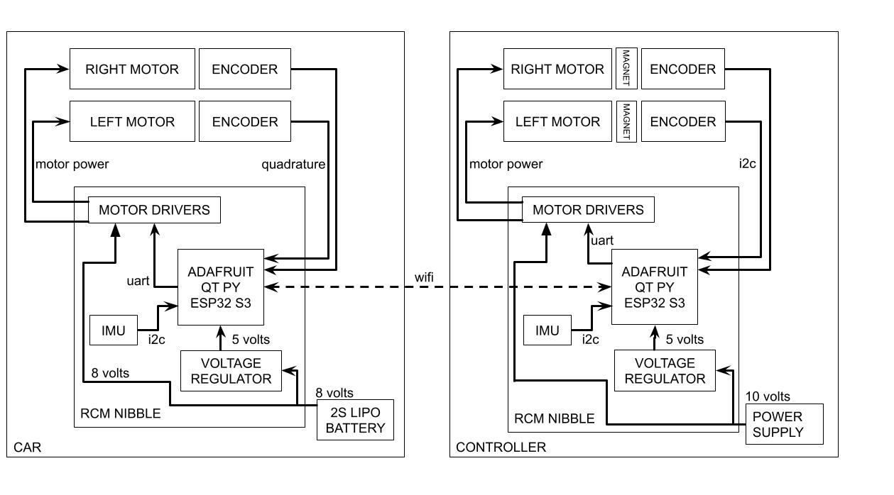
Figure 3. Electronics System Diagram

The controller uses direct-drive Maxon motors for high transparency, and magnetic absolute encoders (as5048b) for their mechanical simplicity.

The car uses geared motors with quadrature encoders. We needed high torque to climb inclines. Requiring continuous rotation ruled out capstan drive and our prototype car with direct drive was extremely challenging to drive in a straight line or any controlled direction.

We used “Nibble” Robot Control Module boards that Joshua had designed a couple of years ago for controlling the motors. They were a bit underpowered for our application since the motors could have handled higher currents than the boards could provide, but they simplified the connection of a battery, motors, and encoders to our ESP32 boards and kept our electronics very small. The Nibble boards contain a voltage regulator, two TMC7300 motor driver ICs, and an IMU.

For our ToF proof-of-concept, we used VL53L0XV2 sensors.

Hardware

Purchased car

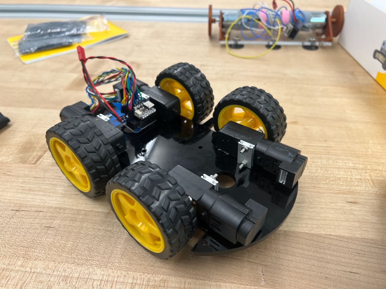
While it may look like we just bought a Smart Robot Car Kit V4.0 from Elegoo and called it a day, the truth is that we only used the laser cut mounting platform, miscellaneous mounting hardware (nuts, bolts), battery, and wheels from the kit. The goal in doing this was to avoid building a car from scratch, which wasn’t relevant to the scope of our project.

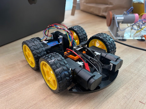
Figure 4. Purchased Car

The Car We Built From Scratch

Figure 5. Small car CAD

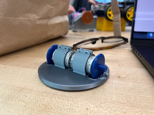
Figure 6. Small car

The goal with this car was to use the HapKit motors in direct drive to have a more transparent impedance signal by avoiding the gearboxes of the other motors. The haptic response felt incredibly transparent (to the point where you could feel small indents in the ground), but the car itself was very hard to control and didn’t lend itself well to going up ramps or pushing objects for… obvious reasons. The magnetic encoders were also incredibly inaccurate, which led to much more jolts and unreliable impedance readings at times. In an alternative world where Stanford was on the semester system, we would’ve tuned/fixed this system to make it work, as there was a lot more potential for good data in this solution.

Controller

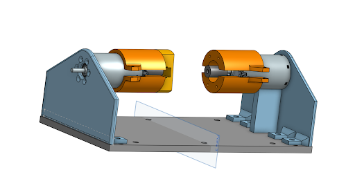
Figure 7. Controller CAD

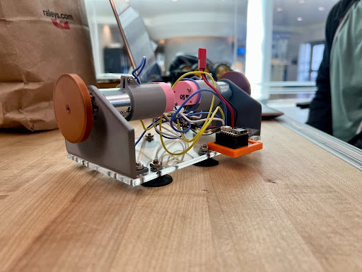
Figure 8. Controller

The goal with the controller was to have an intuitive differential drive system that could transmit left and right-wheel impedance independently. At the beginning of the project, we were also experimenting with position-based controls, which is why we wanted a direct drive system rather than a capstan-based one.

We ended up mounting the Maxon motors in an elevated position to allow for comfortable gripping of the wheels.

Results

Quantitative Results

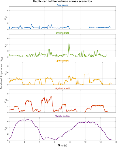
Figure 9. Uncropped/Unfiltered Data

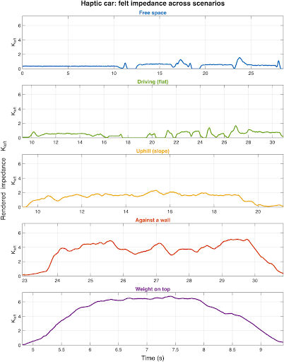
Figure10. Cropped/trimmed to individual trial

In our baseline, free-space case, we can see that we still have some noise and non-zero resistance in the system due to the inertial resistance of the gearbox and wheel of the car. This noise scales up as we drive on flat terrain, and we can see that sometimes we get large peaks in our impedance as the motors struggle to overcome the friction and locking of the gearbox.

On our gentle uphill slope, we can see that our K value increases to 2. Against a wall, it moves up to around 4, but we can see that as the wheels slip, we get big dips before the K-value climbs again. And finally, with the weight on top, we're able to maximize the K-value and get it up to 6.

Qualitative Perception

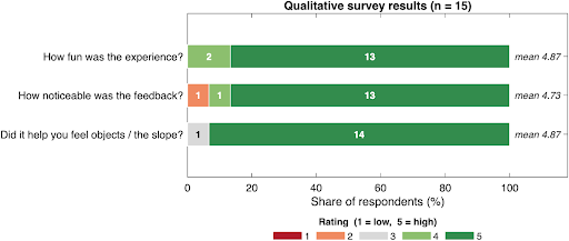
Figure 11. Qualitative survey results Out of the 15 respondents to our survey, we found that most seemed to enjoy the experience (though there might be some bias due to this being a showcase event). One participant noted that they wished that the remote force feedback was stronger, as the weaker force made it hard to discern impedance versus the noise floor.

Controls/Dynamics Analysis

Analysis Objective

The goal of this analysis is to characterize the behavior of the rendered impedance signal, K_left, across driving conditions and determine whether the adaptive haptic controller produces a stable, bounded, and intuitively increasing resistance in harder scenarios. The main question is whether the controller delivers low impedance in free space and on flat ground, while increasing the felt stiffness when the vehicle is loaded, climbing a slope, or contacting an obstacle.

Method

For each scenario, the log data were cropped to a fixed time window corresponding to the relevant portion of the run. The resulting K_left(t) traces were smoothed with a moving average to suppress sample-scale noise while preserving the overall transient behavior. Several metrics were then computed for each scenario: mean, standard deviation, maximum, 95th percentile, and median. To capture transient response shape, rise-time and decay-time proxies were computed when a clear transient was present. The free-space condition was used as the reference for contrast comparisons.

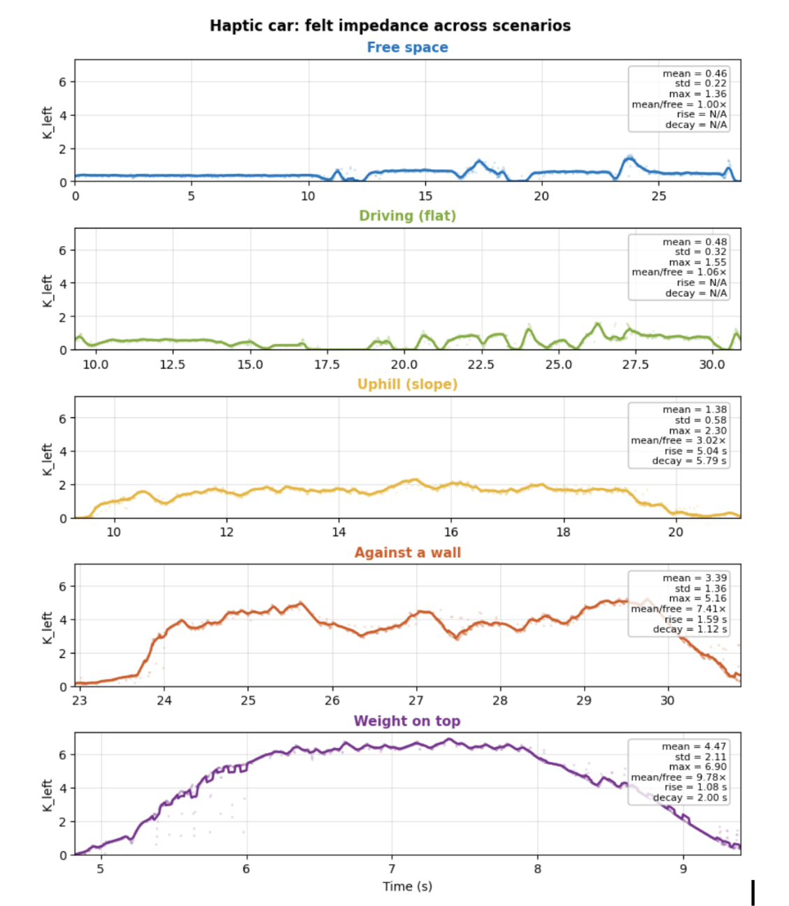
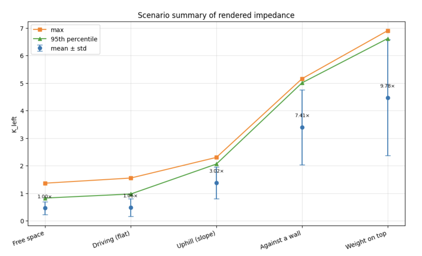
Figure 12. Scenario summary of rendered impedance

Interpretation of the Results

The traces show a clear ordering of impedance across scenarios. Free space produces the lowest average K_left, with only small fluctuations and brief spikes. Flat driving produces a slightly higher and more variable impedance, consistent with small transient load changes from normal motion. Uphill driving shows a sustained increase in K_left, indicating that the controller raises the apparent stiffness when the car experiences more resistance. The wall-contact and weight-on-top cases produce the largest mean and peak values, demonstrating that the controller detects stronger impediment and responds by increasing the rendered impedance substantially. The area under the curve is also largest in the high-load cases, which indicates that the high-stiffness state is not merely a brief spike but persists over a meaningful time interval. The rise and decay proxies are useful for describing how quickly the feedback ramps up when the car becomes impeded and how quickly it returns to baseline when the load is removed.

Control and Dynamics Discussion

This behavior can be interpreted as a bounded adaptive impedance controller. The rendered stiffness is adjusted in response to a mismatch between expected free-space motion and measured vehicle motion. In control terms, this is a form of gain scheduling: the effective stiffness increases when the system detects a larger obstacle or load-related discrepancy, and decreases when the vehicle is free to move. The filtering and rate limiting in the controller act like a first-order smoothing dynamic on the gain update, which prevents rapid switching and helps avoid the unstable oscillations seen in earlier versions of the code. The saturation bounds on K_left are also important because they guarantee that the rendered stiffness remains finite and physically reasonable. Taken together, the results show that the controller creates a useful contrast between free space and resistance while remaining bounded and stable enough for human interaction.

Future Work

Friction was one of the key limiting factors in both cars: when the wheels slipped, the motors weren’t being impeded. Having better tires that increase friction will naturally improve the impedance readings. That being said, the wall scenario is one that won’t be fixed with additional friction, as you can imagine that the car might try to “climb” the wall, so the “wall”/rigid impedance wouldn’t be felt.

For this, we’d like to have implemented the ToF sensor solution that we demonstrated at the showcase. Wall detection with a simple VL53L0XV2 sensor could then be converted to “safety stop” on the car’s forward movement, and the controller could switch to a mode representing the stiffness of the wall.

An additional limitation was controller motor saturation. This set an upper limit on the impedance communicated to the user. Increasing current capacity, for example by swapping the driver IC for a higher-current part or running two TMC7300 channels in parallel per motor, would make space for additional impedance communication capacity.

Further filtration efforts can be applied to impulsive gearbox/encoder data spikes that slip through our current low-pass and motion-gate stages. Additionally, improving wifi connection (perhaps with better hardware) or implementing a last-value-holding when connection is temporarily lost and regained would smooth the resulting gaps without adding latency.

Field testing is the real open question, since everything so far has been bench and showcase work on flat tables, ramps, and a wall. An informal test over rough or cluttered terrain with the operator working partly blind would tell us whether independent left/right load reflection actually adds anything on top of a camera feed in a rescue or exploration setting.

Acknowledgments

We would like to thank the Lab64 makerspace for providing materials and tools.

And of course we are so grateful to the ME327 teaching team.

References

Anderson, R. J., & Spong, M. W. (1989). Bilateral control of teleoperators with time delay. IEEE Transactions on Automatic Control, 34(5), 494–501.

Diolaiti, N., & Melchiorri, C. (2003). Haptic tele-operation of a mobile robot. IFAC Proceedings Volumes (SYROCO 2003), 36(17), 521–526.

Farkhatdinov, I., Ryu, J.-H., & Poduraev, J. (2009). A user study of command strategies for mobile robot teleoperation. Intelligent Service Robotics, 2(2), 95–104.

Farkhatdinov, I., Ryu, J.-H., & An, J. (2010). A preliminary experimental study on haptic teleoperation of mobile robot with variable force feedback gain. IEEE Haptics Symposium 2010, 251–256.

Lee, D., & Spong, M. W. (2006). Passive bilateral teleoperation with constant time delay. IEEE Transactions on Robotics, 22(2), 269–281.

Li, W., Ding, L., Gao, H., & Tavakoli, M. (2016). Kinematic bilateral teleoperation of wheeled mobile robots subject to longitudinal slippage. IET Control Theory & Applications, 10(2), 111–118.

Li, W., Ding, L., Liu, Z., Wang, W., Gao, H., & Tavakoli, M. (2017). Kinematic bilateral teledriving of wheeled mobile robots coupled with slippage. IEEE Transactions on Industrial Electronics, 64(3), 2147–2157.

Niemeyer, G., & Slotine, J.-J. E. (1991). Stable adaptive teleoperation. IEEE Journal of Oceanic Engineering, 16(1), 152–162.

Rösch, O. J., Schilling, K., & Roth, H. (2002). Haptic interfaces for the remote control of mobile robots. Control Engineering Practice, 10(11), 1309–1313.

---

Appendix: Project Checkpoints

Checkpoint 1

Here you will write a few paragraphs about what you accomplished in the project so far. Include the checkpoint goals and describe which goals were met (and how), which were not (what were the challenges?), and any change of plans for the project based on what you learned. Include images and/or drawings where appropriate, using a command like this:

Michael

Designed / 3D printed / laser cut mounting / brackets for controller. Initial bracket design is too low to the ground; brackets will be extended (see third figure below) to allow user to 'grasp' controller wheels all around.

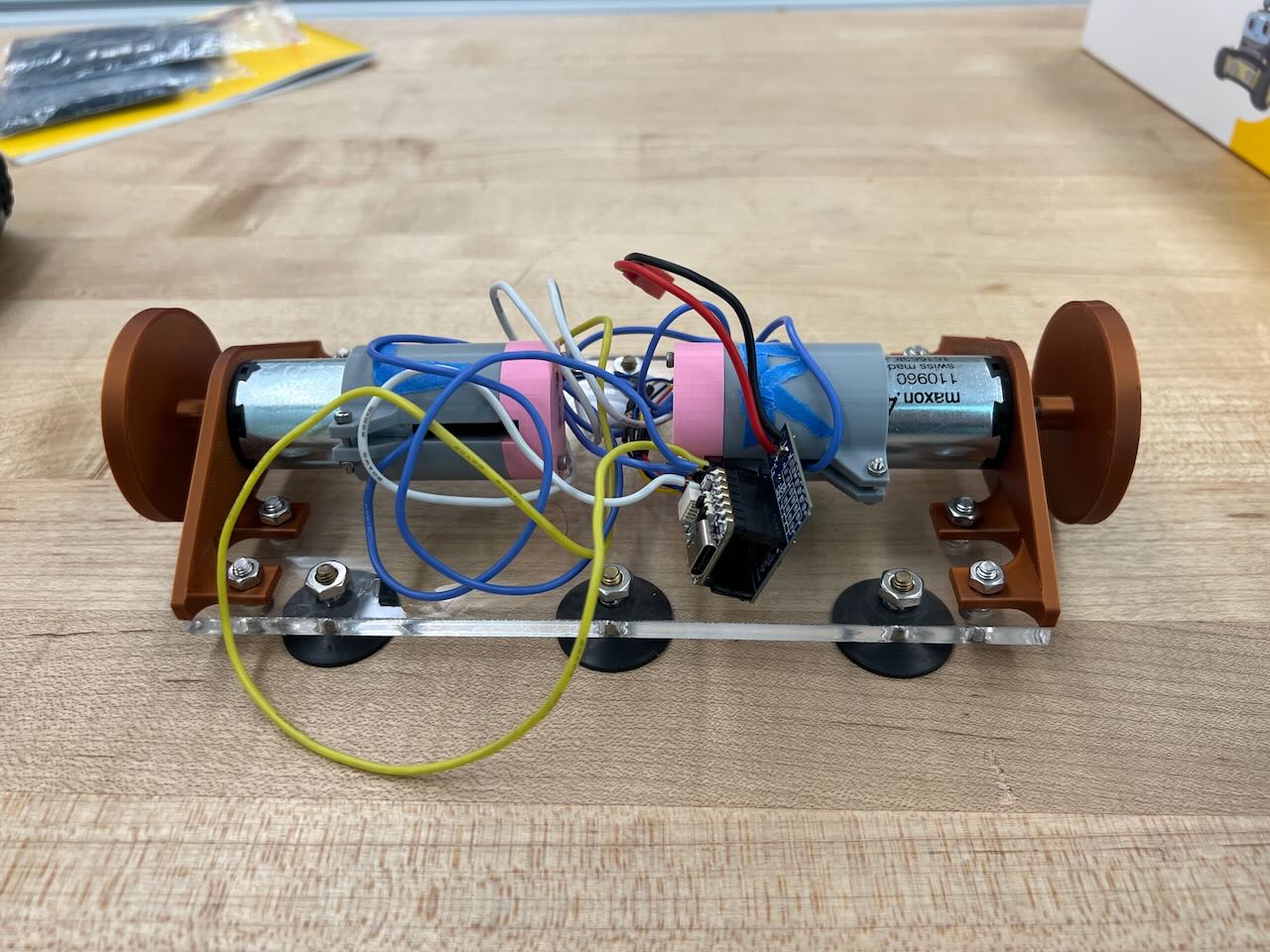
Figure C1.1. Top view of controller

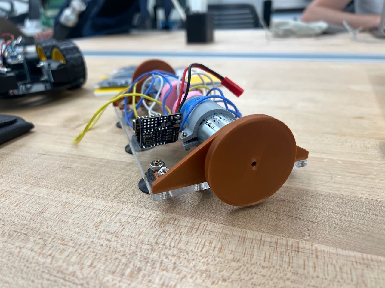
Figure C1.2. Close-up of controller

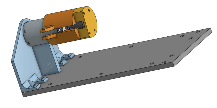
Figure C1.3. Revised bracket model

Brian

Did mechanical assembly for the car frame including mounting motors as well as the battery. No issues so far; the car is in a testable state.

Figure C1.4. Isometric view of car assembly

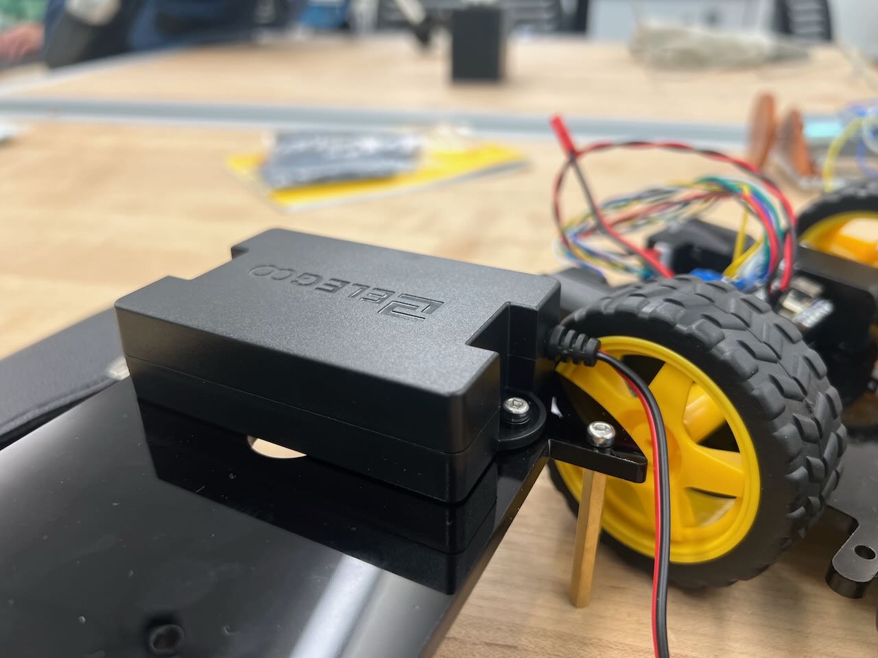
Figure C1.5. Car battery installation

Joshua

I tested software for wifi communication, motor control, and encoder reading. I electrically connected the motors and encoders, and I made 3d printed parts for connecting magnetic encoders to motors. We’re using this software template for esp32-based robots https://github.com/rcmgames/rcmv2. We’re using these circuit boards https://github.com/RCMgames/RCM-Hardware-Nibble.

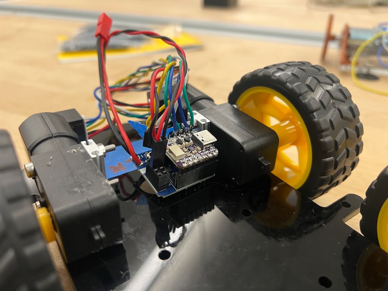
Figure C1.6. Car electricals

Enrico

Software controls: Calibrated motors, Implemented preliminary unilateral position to position and position to velocity control. So far, no issues. Code: https://github.com/ME327-2026-team1.

Checkpoint 2

Here you will write a few paragraphs about what you accomplished in the project so far. Include the checkpoint goals and describe which goals were met (and how), which were not (what were the challenges?), and any change of plans for the project based on what you learned. Include images and/or drawings where appropriate.

Michael

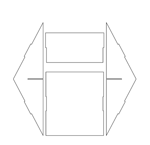
Figure C2.1. Original ramp proposal sketch

Figure C2.2. Original ramp proposal render

Preliminary work has begun on ramps, though we’re quickly realizing we need something that: - Doesn’t deflect under load - Doesn’t slip when the car drives up it This laser cut ramp was a decent concept, but then I thought… what if we didn’t need to do that?

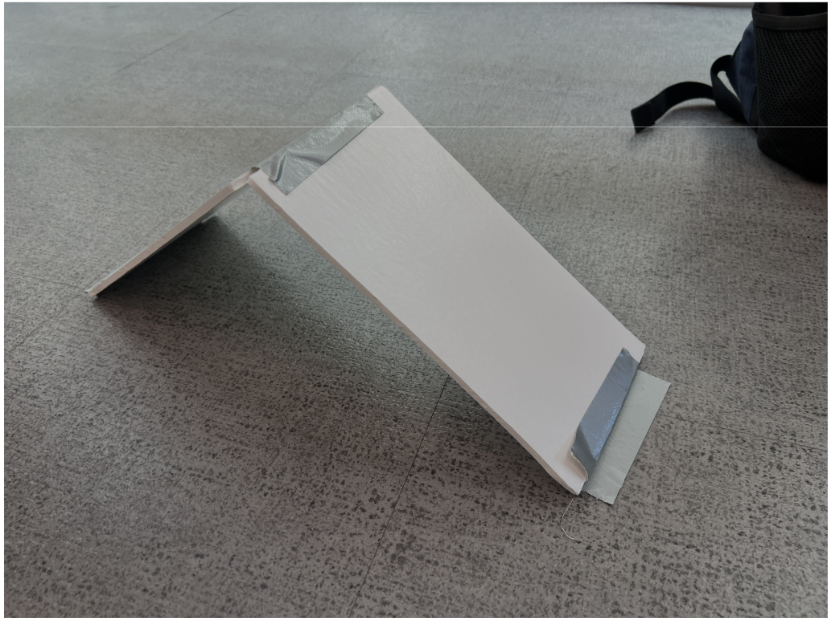
Figure C2.3. Simplified ramp

This duct tape-foam core setup will avoid all laser cutting and assembly on something that really isn’t the focus of the expo.

Brian

Software controls: setting up alternative impedance measurement method reliant on delta between free space wheel motor velocity and operational wheel motor velocity. The idea is the user feels a force on the controller when the motors are 'struggling' (large delta between free space velocity and current).

Joshua

Worked on cad and electronics for direct drive car (see below). We will test to see whether the transparency and transmitted impedance is significantly higher compared to our current off-the-shelf car assembly (which has gear reductions for the motors).

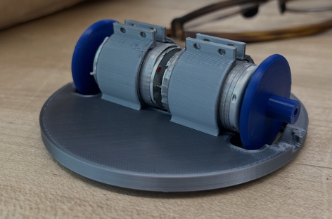
Figure C2.4. Alternative direct drive car

Enrico

Software controls: Implemented IMU sensor reading, including calibration and filtering. This is the original impedance measurement method which is limited to changes in terrain slope (inclination). We may combine both IMU-based feedback and Brian's delta velocity approach if we deem performance to be best in such a configuration.