

2026-Group 10
Haptic Hunt: a pantograph rendering of complex shapes
Project team member(s): Ana Aranzola, Brandon Wong, Chiara Cementon, Sunny Li
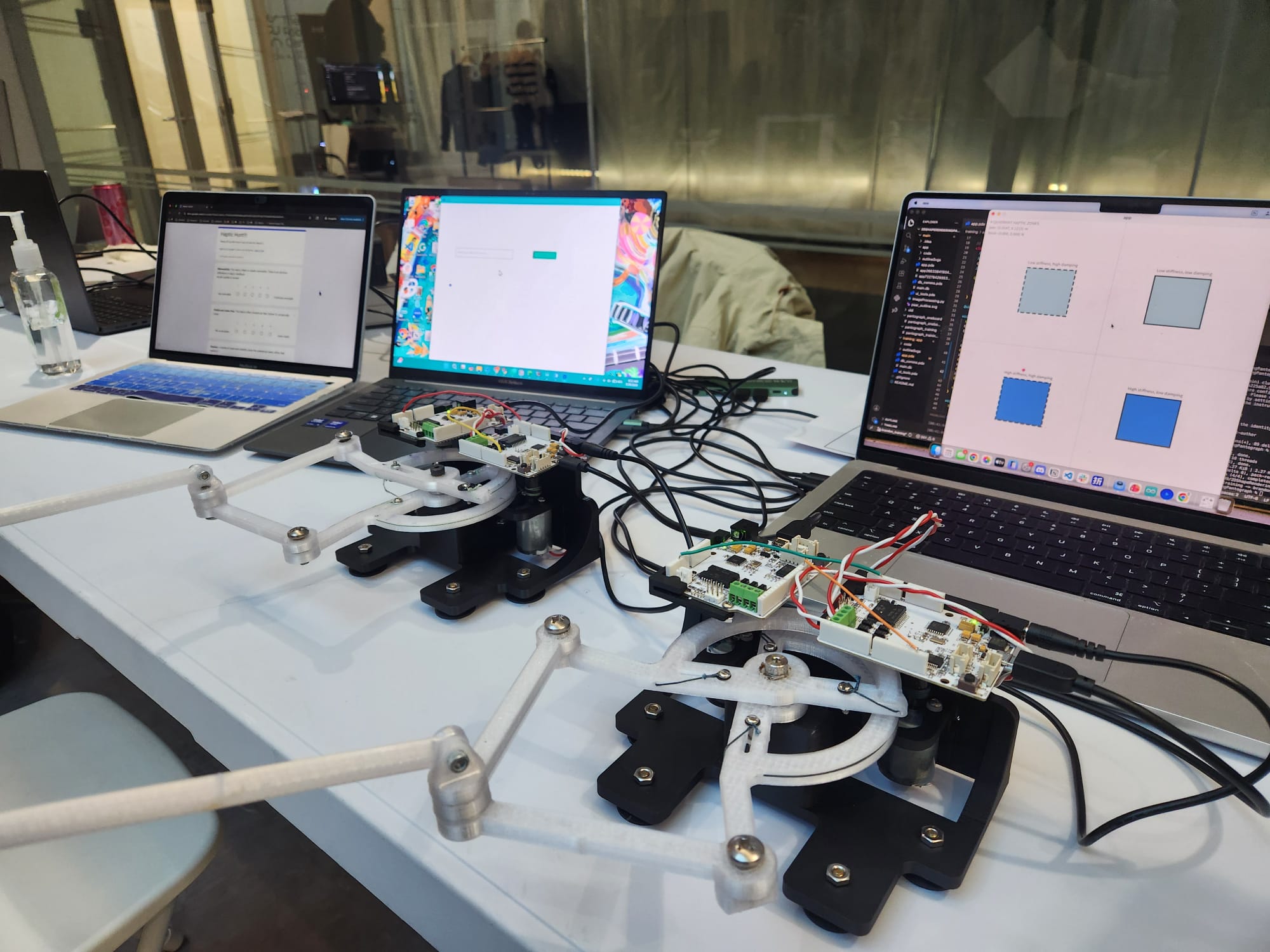
Haptic Hunt is a haptic device game that uses kinesthetic feedback and minimal visual cues to allow users to feel and then guess the outlines of common 2D shapes with distinguishing geometric features, such as a fish, bell, and mushroom. The user traces the shapes through a four-bar pantograph, and the firmware renders a virtual wall along each shape�s boundary with per-shape stiffness and damping so that different shapes feel different to the touch. Based on concepts from the lecture, we incorporated pantograph forward kinematics, the Jacobian transpose for force-to-torque mapping, and a proxy-based force model that slides along the polygon boundary to keep the rendered force direction stable. At the open house, 20 participants tried the device and rated it 4.65 for noticeability, 4.70 for stability, and 4.40 for realism on a 1-5 scale, with all participants reporting that it was fun. In the future, the project can be extended by running a controlled study with and without haptic cues to test whether stiffness and damping actually help users identify shapes, and by adding textural feedback as a further comparison.
On this page (hide)
- 1. Introduction
- 2. Background
- 3. Methods
- 4. Results
- 5. Future Work
- 6. Acknowledgments
- 7. Files
- 8. References
- 9. Appendix: Project Checkpoints
- 9.1 Checkpoint 1
- 9.2 Checkpoint 2
1. Introduction
While spatial awareness is mostly guided by vision, touch is an important secondary cue that helps individuals form mental images of spaces and geometries. Understanding our physical environment through a tool rather than touch alone can be applicable to teleoperation, VR/AR, and as a tool for visually impaired people. For instance, in teleoperation in extreme environments such as space or underwater exploration, an operator would greatly benefit from haptic feedback of objects they�re manipulating. Our group sought to study how well users can identify shapes through kinesthetic feedback alone and if added cues such as texture and realistic stiffness will aid in this process.
Our device is a pantograph that allowed us to test shape discrimination in two dimensions. A pantograph enables both 2-D motion tracking and force feedback. Thus, with this device we could encourage users to trace the outline of a shape from the outside (by applying a virtual wall inside the shape). We chose to have users trace the outline of a shape from outside (rather than inside), to mimic the way a shape feels in the real world. We were specifically interested in whether textural or differing stiffness feedback would help with shape identification.
2. Background
2.1 2D haptic devices
2D haptic devices have found applications in field such as surgical simulation, accessibility technology for the visually impaired, and virtual reality interfaces. Haptic devices face a common tradeoff between �transparency� (i.e. objects being rendered by the device feeling real, and free space feeling free) and stability. [2] In rendering virtual objects in two dimensions, pantographs are found to be fairly transparent and stable due to their low inertia and direct drive linkage design. It has dynamic range, resolves small displacements and has a high frequency response. [3] For these reasons, we use a pantograph to render 2D shapes.
2.2 Shape discrimination
Shape tracing is a largely kinesthetic method to determine shapes through touch, while texture/softness is cutaneous. Previous work shows that a combination of tactile and kinesthetic feedback creates more realistic virtual environments for shape discrimination. [4] It has been discussed in the literature that haptics can help users discriminate shape but compared to vision it is effortful and takes time. [5, 6, 7] In [8] it is shown that tactile landmarks (e.g. anomalies in a map) helped participants form stronger maps in memory. In our study, shapes, although complex, are chosen with distinguishing features (such as the size of a fish's tail being exaggerated) to help participants distinguish between the shapes. Our work attempts to extend this work in cognitive maps to complex shape outlines - can users recognise complex shapes through touch alone if aided by both kinesthetic and cutaneous feedback?
2.3 Rendering surface textures
Relevant to this work specifically are the use of spring-damper models to simulate walls and adding texture to walls using dampening or stiffness. There are many examples in the literature that explore stiffness and damping as texture rendering methods. (We include references to some review papers here: [9, 10]). In particular, we were interested in studies that used variable stiffness and damping to help with realistic virtual object rendering.
Reference [11] uses the NOVINT Falcon haptic device to render object surfaces in three dimensions. Most notably, the researchers render forces using a spring-mass damper model with virtual stiffness related to the elastic modulus of the object at the point of contact. This study only performs a brief user study with hapto-visual rendering and doesn�t expand too much on user perception of stiffness or texture. The aim of our study is to understand experimentally if users can perceive these variable stiffnesses well.
To ensure our device would be stable, we use a simple velocity-dependent damping to render a binary difference in texture - slippery and sticky. The authors of reference [12] show that the force exerted by different textured surfaces on the fingertip is proportional to finger speed. While damping is not the only contributor to surface roughness perception, other effects can produce device instability [13] and stability was the ultimate priority for our application. In future iterations of this study, it would be beneficial to use more modern texture rendering models, with a focus on not introducing too much instability to the system.
3. Methods
3.1 Hardware Design and Implementation
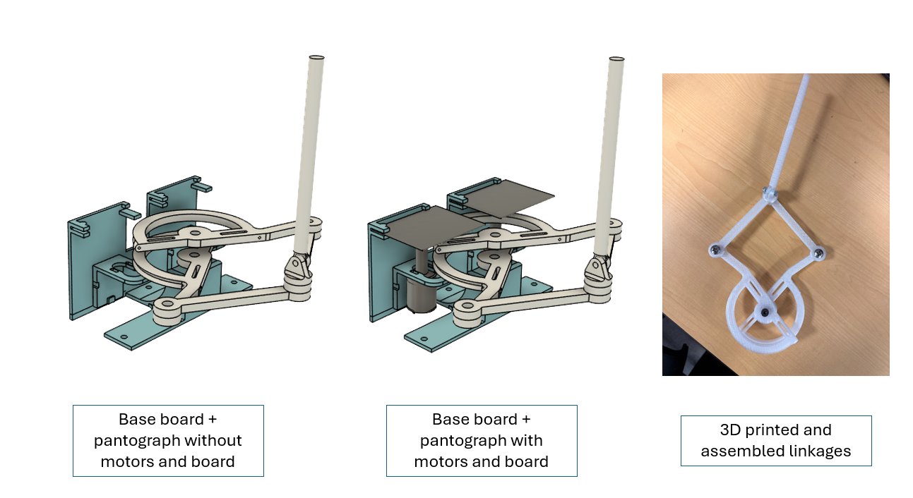
A pantograph is a mechanism that allows for 2 degrees of freedom in a 2d plane. In contrast to a robotic arm with one actuator at the shoulder and one actuator at the elbow, a pantograph has the advantage of keeping both motors fixed in place at the base of the mechanism, greatly reducing the inertia of the system. In general, 2d pantographs can be described as a 5 bar linkage, with one �bar� being the fixed relative position between the two base actuated joints. For convenience and kinematic simplicity, we chose this 5th �bar� to be length 0�that is, the two drums of the capstan drives to be concentric�and the lengths of the 4 other bars of the linkage all to be 10cm.
The core components were reused from two Hapkits, namely the boards (for the magnetic encoders), capstans with magnets, and the motors. The drums were redesigned to have a 180-degree range of motion, with a slightly smaller radius than the Hapkit drum, and an overlapping axis for the center rotation of the sectors.
In addition to the two actuated position degrees of freedom, we added a passive universal joint to the end effector for two additional rotational degrees of freedom for the user�s �pen� interface. The pantograph handle resembles a pen that allows users to get a comfortable grip and simulate a real "drawing" experience. This is similar to the passive rotational degrees of freedom on the 3DSystems Touch.
We 3D printed the linkages in PETG using an Ender 3D Printer. One notable point is in the friction of the joints. Each joint had one hole that was friction fit for the screw threads to bite into directly, and the other hole(s) involved in the joint were press fit with a lubricated bushing, which could rotate freely around the screw. (Both the lubricated bushings and the screw threads lock fits were assembled by softening the plastic with a soldering iron). The other end of the linkage was intentionally left to be hand-tapped to secure the screw with no additional nuts. The base has spaces to fit rubber suction cups, and near the motors, it has holes where zipties will secure the motors in place.
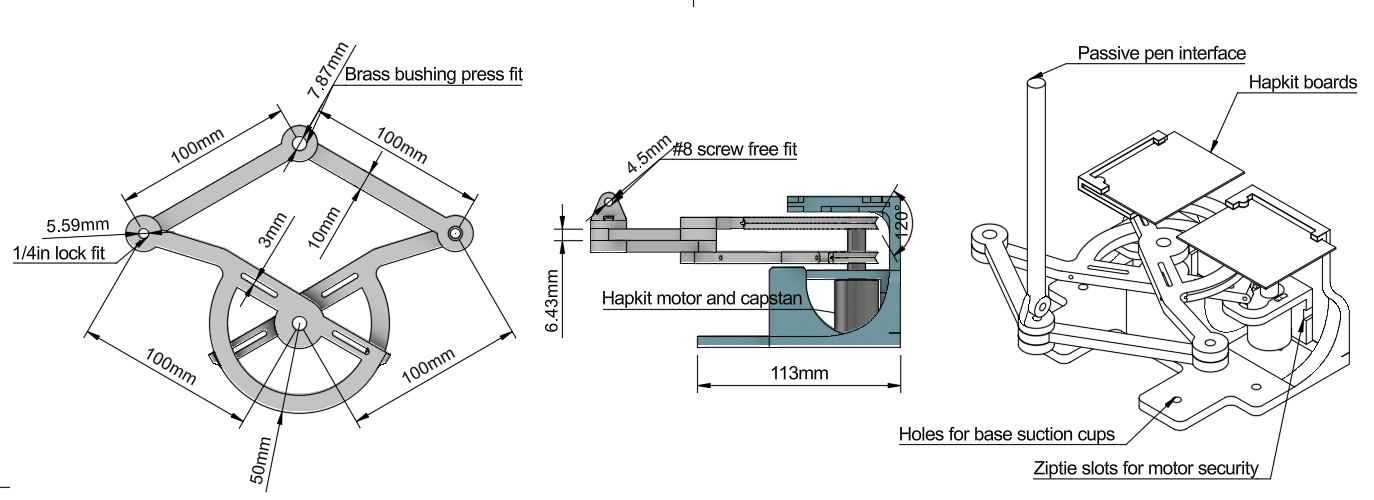
Fig 1: Dimensioned drawings: top down view of the linkage geometry, side profile of the linkage and grame, and orthographic view of the entire system.
The frame was perhaps the most difficult part of the hardware design. It needed to support the pantograph linkage base, the motors, and the hapkit boards in place with enough stiffness to prevent tipping, flexing, or vibration issues. Additionally, the frame needed to stay out of the way of the linkage workspace, which was more difficult than expected because we initially forgot to account for the non-negligible presence of fasteners sticking out. Another unexpected problem arose when the boards were arranged in a way that blocked access to one of the USB ports. In the final design, the boards are rearranged to access both ports, and other components of the base were redesigned to reduce friction and improve mechanical (tipping) stability. The final base was printed from PLA on a Bambu.
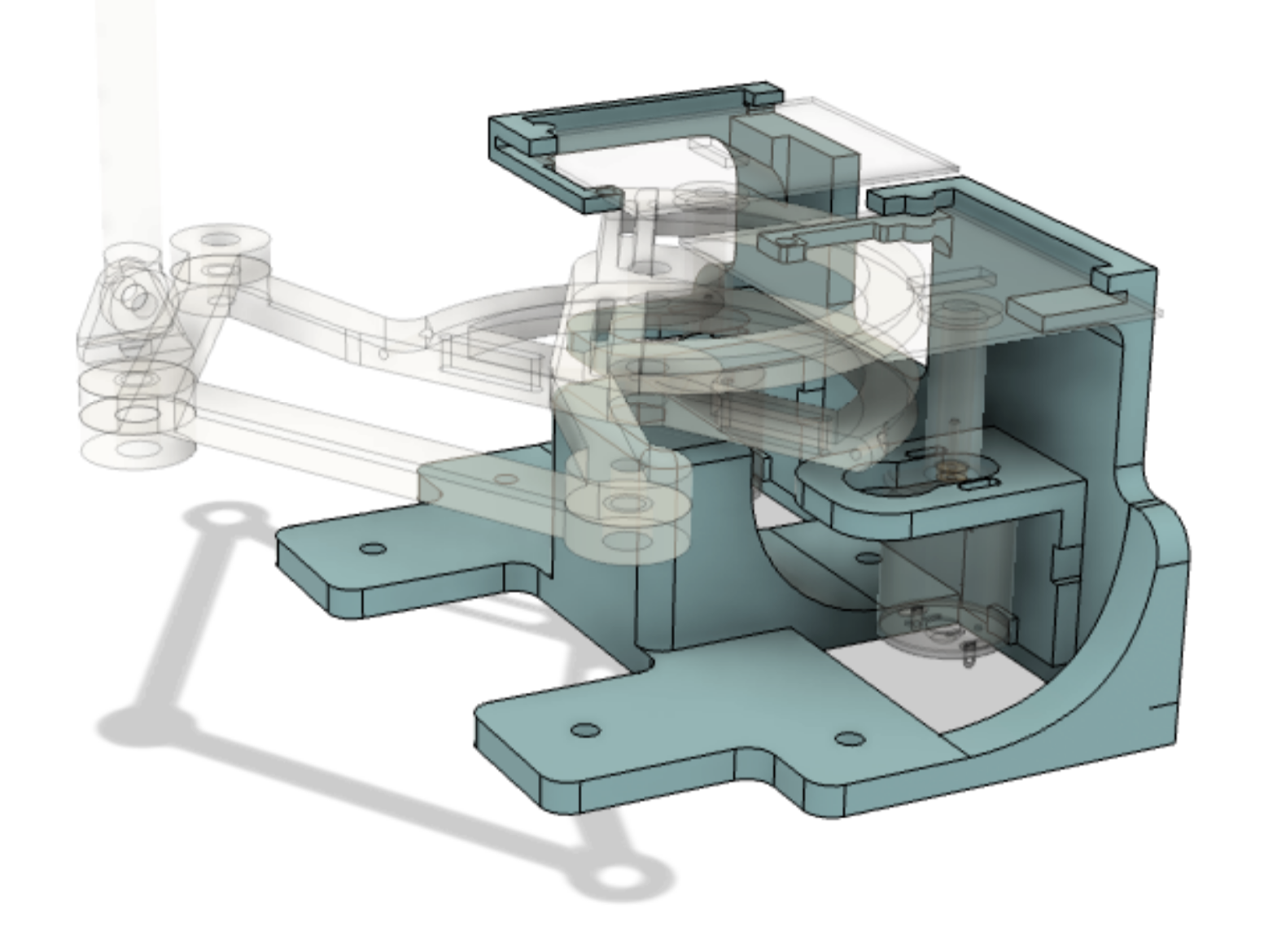
Fig 2: The frame holding the linkage, motors, and boards together while avoiding interference with the linkage workspace
Finally, the motor mounts, cable threading, and capstan winding were all assembled in a similar manner as the Hapkit, with the addition of zipties to further secure the motors to the base. The Hapkit boards were mounted with a similar slotting mechanism as the Hapkit, with an additional 3mm screw to prevent the board from sliding out accidentally
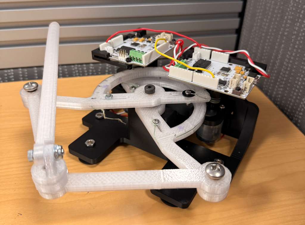
Fig. 3: Final pantograph assembly
3.2 System Analysis and Control
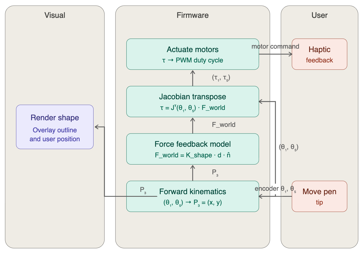
System Diagram
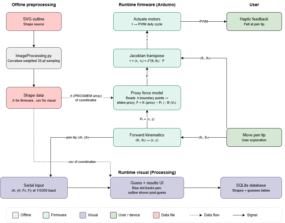
Fig 4: System diagram showing the components of our system and how data flows through the components.
Direct Kinematics
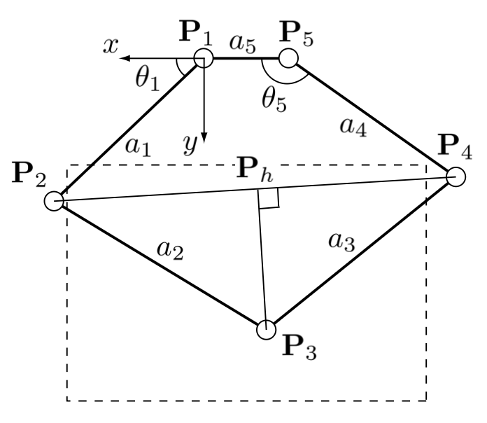
To render force feedback in the correct direction and at the correct location, the firmware needs to know where the pen tip is in 2D Cartesian space at each loop iteration. The only sensors available are the two motor encoders at the base, so we use forward kinematics to map the two measured joint angles (θ₁, θ₅) to the end-effector position P₃ = (x₃, y₃). See figure below for a general 5-bar linkage [1].
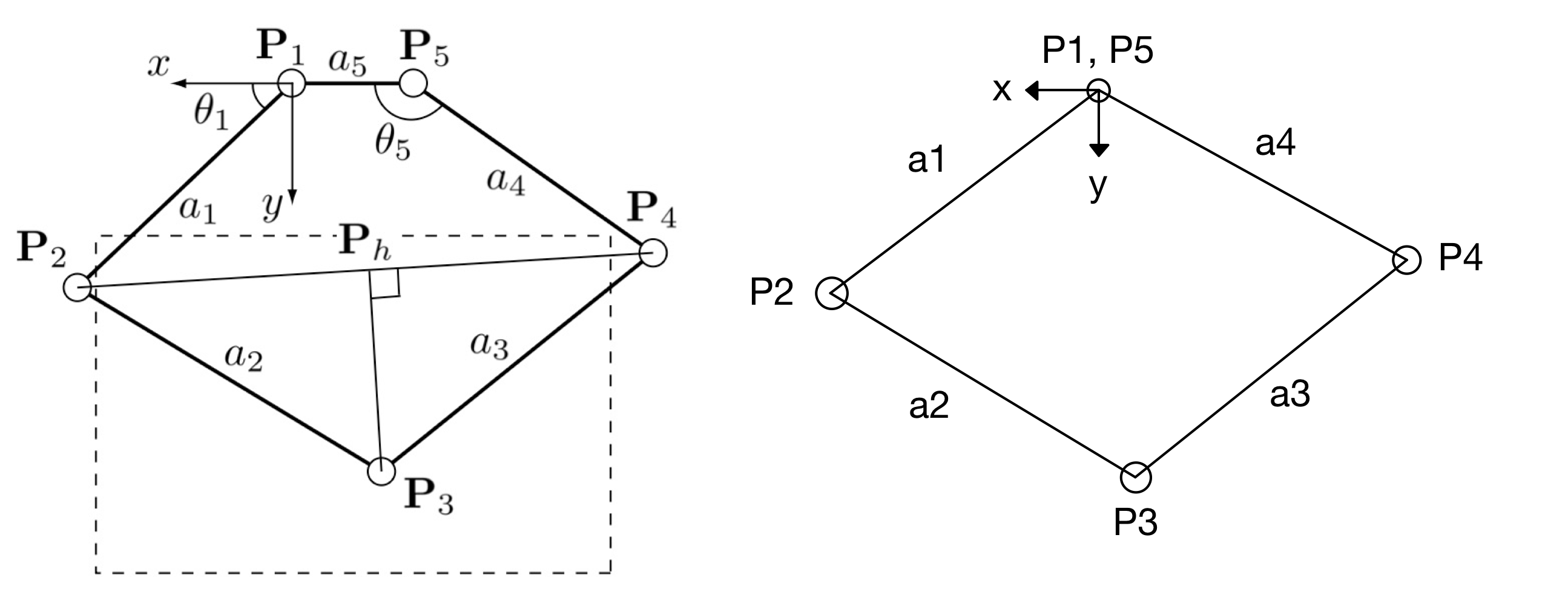
Fig 5: Traditional five-bar linkage (left) and our modified four-bar linkage (right).
Our linkage is a modified five-bar pantograph with the two motors placed at the same x-y location (a₅ = 0), which gives us a wider horizontal workspace than the standard configuration. Following the geometric approach of Campion et al. [1], we treat P₃ as the tip of the triangle P₂P₃P₄, where P₂ and P₄ are the elbows directly driven by the two motors. The derivation proceeds in the following steps:
- Compute the elbow positions P₂ and P₄ directly from θ₁ and θ₅, since each elbow lies at the end of a link directly connected to the motor.
- Find the distance between P₂ and Pₕ using the right triangles P₂PₕP₃ and P₄PₕP₃.
- Compute the altitude ‖P₃ − Pₕ‖ by the Pythagorean theorem.
- Find the coordinates of the base of the height (Pₕ) from P₃ that's on the segment connecting P₂ and P₄.
- Step perpendicular to P₂P₄ from Pₕ by that altitude, choosing the sign convention that places P₃ in the "elbow up" half-plane (the configuration the device actually operates in).
The full derivation, including the resulting closed-form expressions for x₃ and y₃ in terms of θ₁ and θ₅, is shown below.
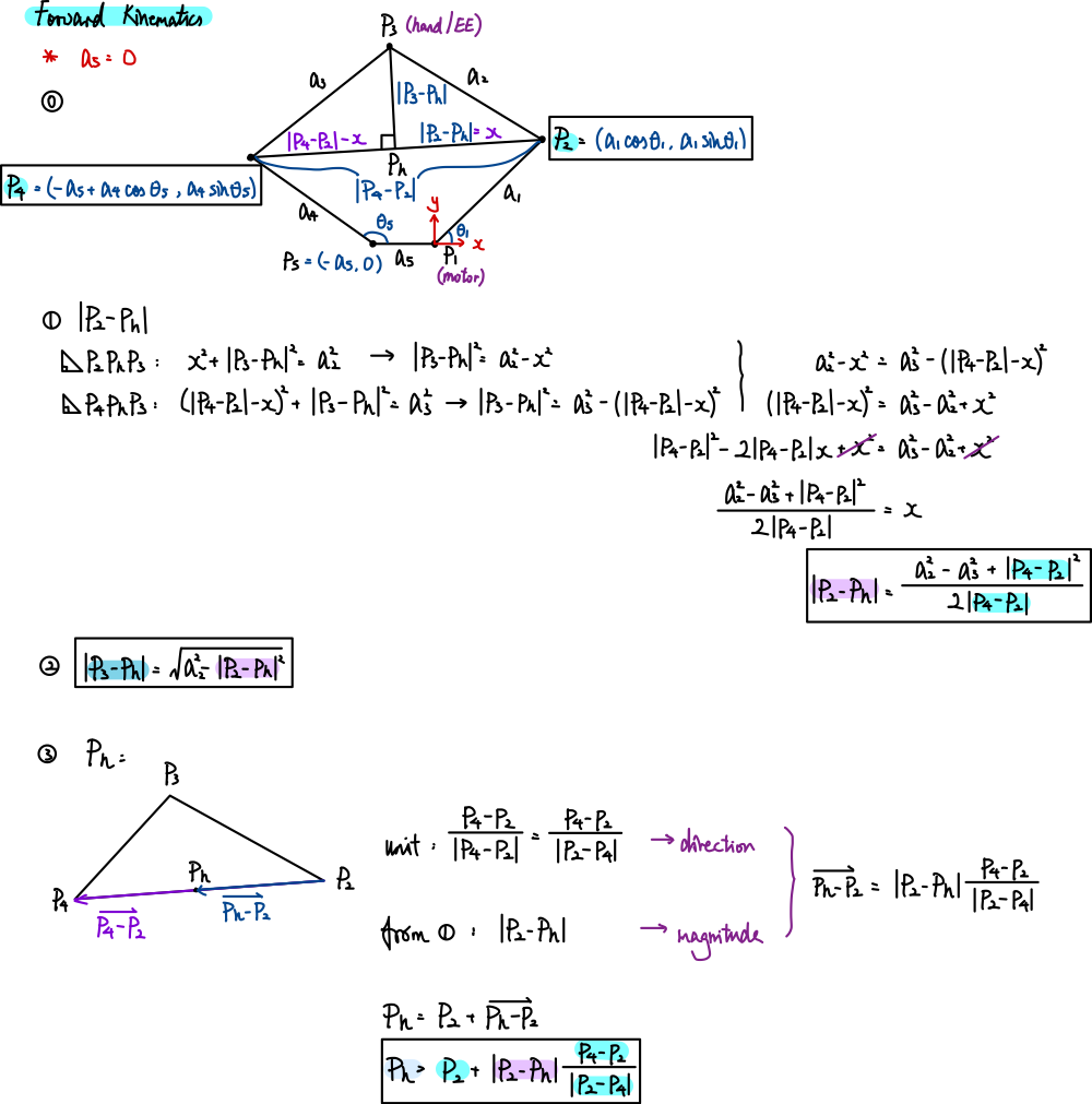
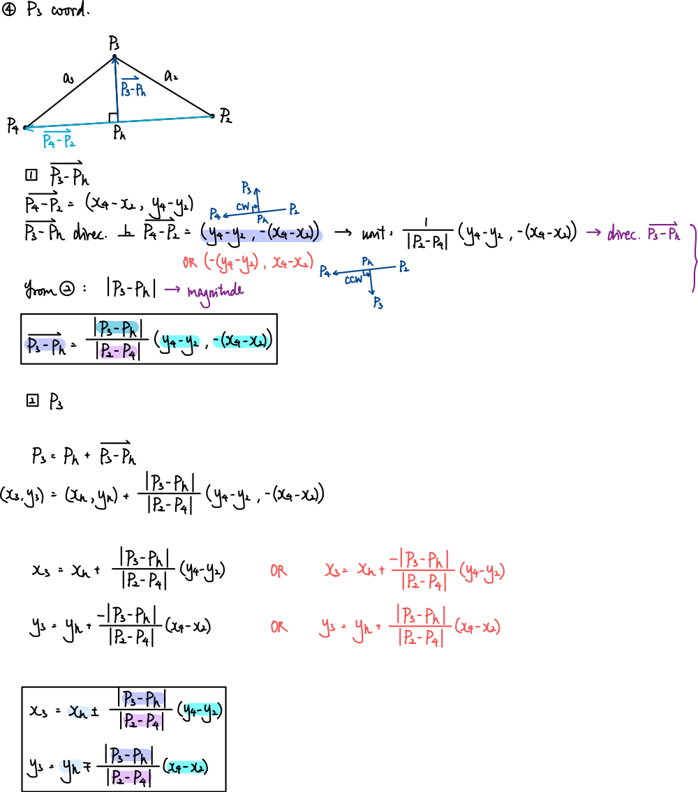
Fig 6: Forward kinematic derivation.
With this forward-kinematics model, given a sensor reading on each loop, the firmware can compute the pen tip's (x, y) position in real time, which is needed for the force-feedback rendering described in the later sections.
Differential Kinematics
Forward kinematics gives us where the pen tip is. To turn the desired force from the force-feedback model into commands the motors can execute, we need the Jacobian. The Jacobian relates joint-angle changes to end-effector displacement, and its transpose maps a Cartesian force at the pen tip to the two motor torques required to produce it: τ = Jᵀ � F. This is the step that closes the loop from the force-feedback model back to the actuators.
Because x₃ and y₃ are built up through a chain of intermediate quantities (P₂, P₄, d = ‖P₂ − P₄‖, b = ‖P₂ − Pₕ‖, h = ‖P₃ − Pₕ‖, Pₕ), the partial derivatives ∂x₃/∂θᵢ and ∂y₃/∂θᵢ are computed by the chain rule applied through each of those intermediate quantities in the same order as the forward-kinematics derivation. We follow the chain-rule expressions in Campion et al. [1]; the Jacobian and its set of equations are shown below.
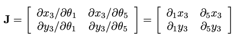
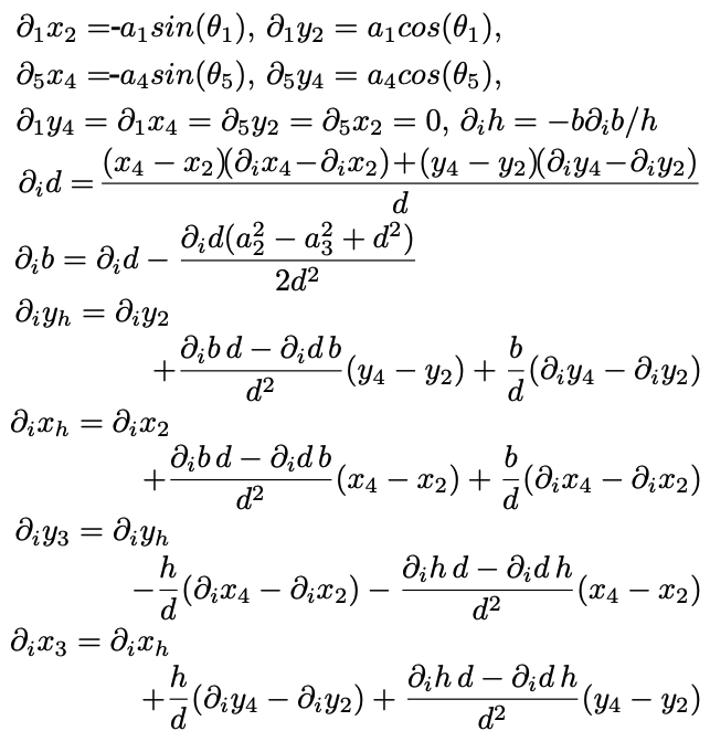
Fig 7: Jacobian equations.
Once the Jacobian is evaluated at the current configuration, the torque required from each motor to render a force F = (Fₓ, F_y) at the pen tip would be τ = Jᵀ � F. The Hapkit board then converts its torque to a motor PWM command using the transmission mechanism relation (Tₚ = F � rₕ � rₚ / rₛ) we used in the homework assignments. This completes the sensors-to-actuation loop: encoder reading → forward kinematics → pen-tip position → [force-feedback model] → F → Jᵀ → motor torques → PWM → motor command.
Firmware

Fig 8: Electronics schematic showing how our system is wired.
The firmware runs on a single Arduino microcontroller (Board 5), which reads both MR sensors (its own on A3 and Board 1's signal jumpered into A2 ) and drives both motors via PWM and direction pins, eliminating inter-board communication delay. At every loop iteration (~1 kHz), the two sensor readings are converted to joint angles and passed through the forward kinematics solver to find the pen tip's 2D Cartesian position (xh,yh)
Controls Analysis
This section describes the firmware-level controls system: how forces are computed from the pen-tip position, how the system parameters were chosen against the closed-loop stability boundary, and how signal filtering and proxy-motion limits were tuned to keep the rendered force smooth and stable. The specific parameters were chosen experimentally by increasing each parameter until instability or perceptible noise emerged, then backing off.
Force Feedback. To determine the forces felt by the user, we experimented using different force models. First we used a simple force computation, but the force direction snapped abruptly at corners, pulling the user in unintended directions. Therefore, we also tried implementing a segments-based computation that would round the corners to avoid snapping whenever the shape had angles at or below 90�. This method found the two nearest edges and blended their forces using inverse-square weighting. However, this introduced the risk of jumping segments. Lastly we tried a traditional proxy-based computation, which we ultimately decided to use, as it made the shape more noticeable, decreased the jumps across thin features, and users in preliminary tests found shape features more distinguishable.
How the traditional proxy-based force model works: In free space, forces will be 0. We tried implementing a gradient force field that would pull the user into the shape. However, preliminary tests showed that users confused the force from the pull with the force from the actual shape, so we decided to keep the free space force-free. Whenever the user crosses the boundary of a shape, the proxy model uses the previous pen tip position (xhprev, yhprev) to determine the boundary crossing point and initialize the proxy on the wall.Then, the saved positions (xproxy, yproxy) are used to calculate the forces
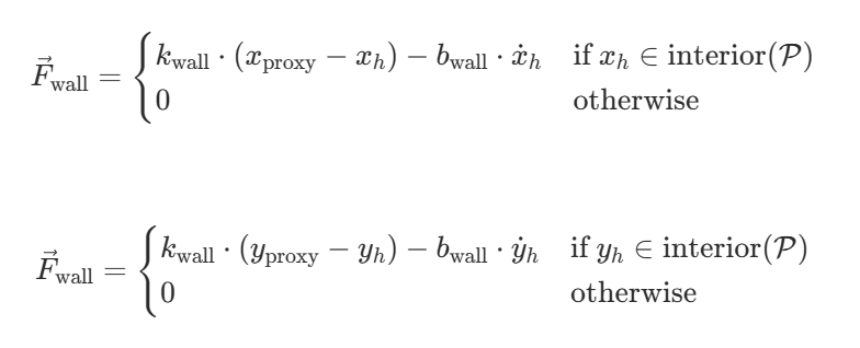
Fig 9: Force computation equations.
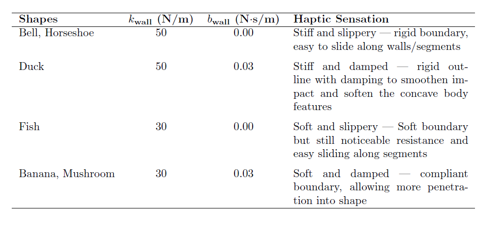
Table 1: Stiffness and damping coefficients of different shapes
For the stiff and slippery shapes we chose to do no damping to increase the perceived sharpness and a stiffness of 50 N/m, as it was the maximum stiffness we could implement before our device became unstable. For the soft and damped case, we chose 30 N/m as the lower stiffness since it still allowed for noticeable resistance while being distinguishable from the higher stiffness used for the stiff shapes. The highest damping we could use was 0.03 Ns/m before the system exhibited instability
The torques are then calculated using the transpose Jacobian and sent to the motors as PWM signals. The motors respond and the user feels force from the motors.
Signal Smoothing and Stabilization. We implemented several control strategies to ensure our system worked smoothly. First, a single Arduino microcontroller was used to control the motors and read positions. We had previously tried using two microcontrollers, one for each motor, but this resulted in significant communication delays that decreased the noticeability and smoothness of our device. For this case, when the pen was stationary, the position estimate exhibited instability and unexpected jumps. Additionally, when sliding along the walls, there would be some experienced oscillation. We solved this problem by using only one microcontroller. Although this decreased the torque output of our motors (now the motor driver had to drive two motors rather than one), we decided this was better than having a �jumpy� system.
Additionally we implemented velocity and force filters to mitigate noise and instability with raw data, such as the instability at rest we had previously encountered. Firstly, we added a velocity clamp so that if velocity exceeded 0.5 m/s it would disregard it and set it equal to zero instead. This outlier is then attenuated by the subsequent low-pass filter, which helps smooth out the noise in velocity by keeping 95% of the old value and only 5% of the new one. Similarly, we integrated a force low-pass filter that kept 70% of the previous forces. This made the system and experience feel very smooth with no shakiness as we slide along the walls or whenever there were any unexpected serial communication delays. Lastly, we added a proxy sliding restriction to stabilize the proxy. Since our proxy was able to slide along the segment it was located on, we restricted this movement so that it would not jump too quickly or skip segments if the movements were very fast. Per loop, the proxy could only move 0.5, or halfway across the current segment, in each direction. These parameter values were determined empirically through iterative testing

Fig 10: Smoothing + stabilization equations.
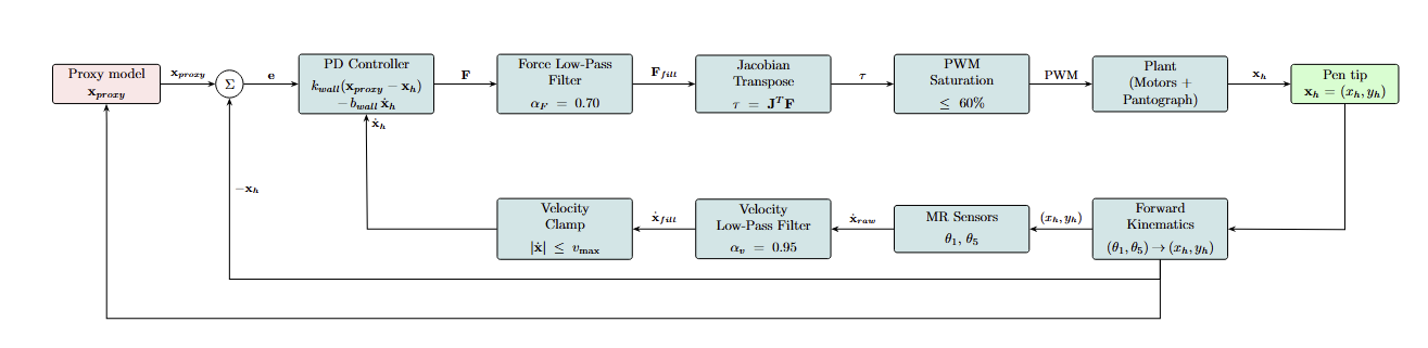
Fig 11: Controls feedback loop diagram
3.3 Graphics and User Interface
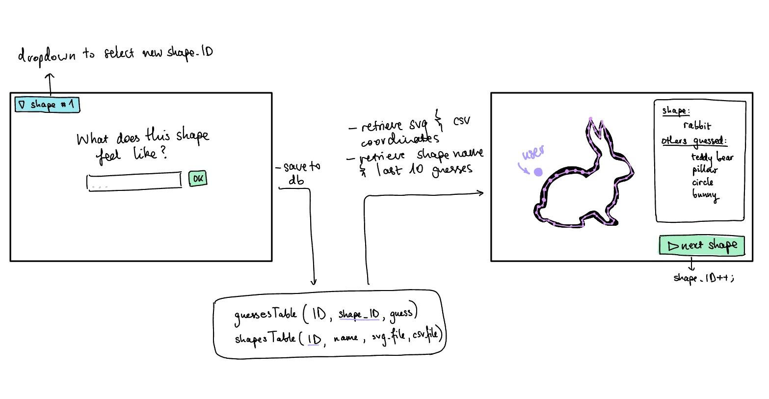
The visual part of Haptic Hunt is a Processing sketch that turns a shape into firmware-readable data offline, runs the game, and logs guesses to a local database.
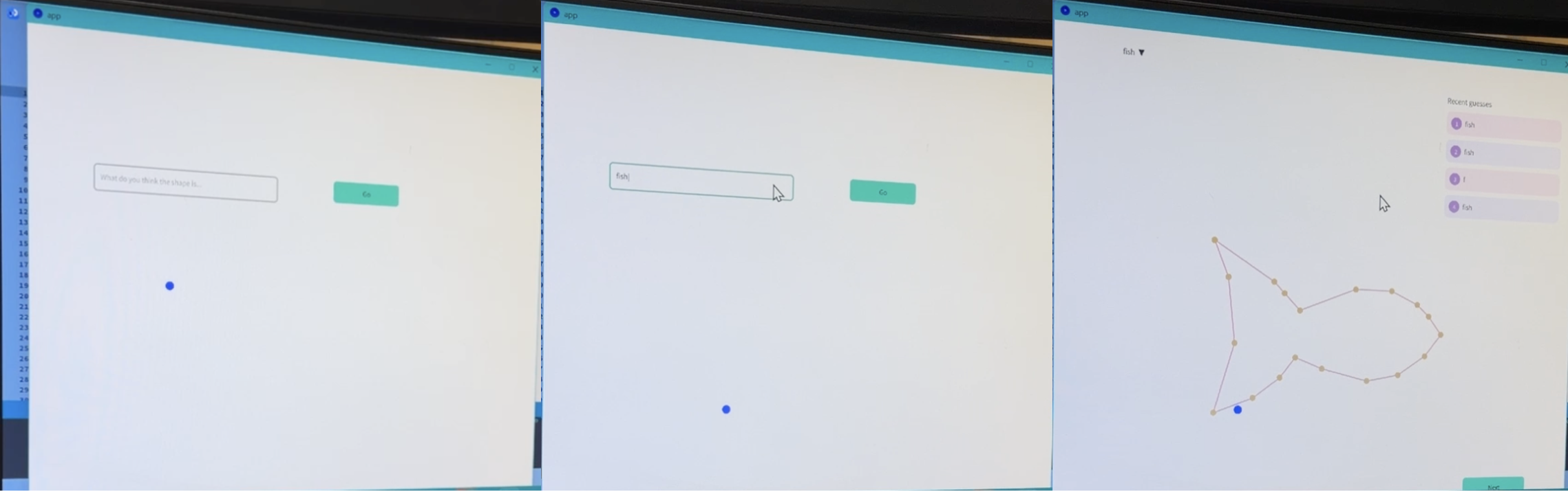
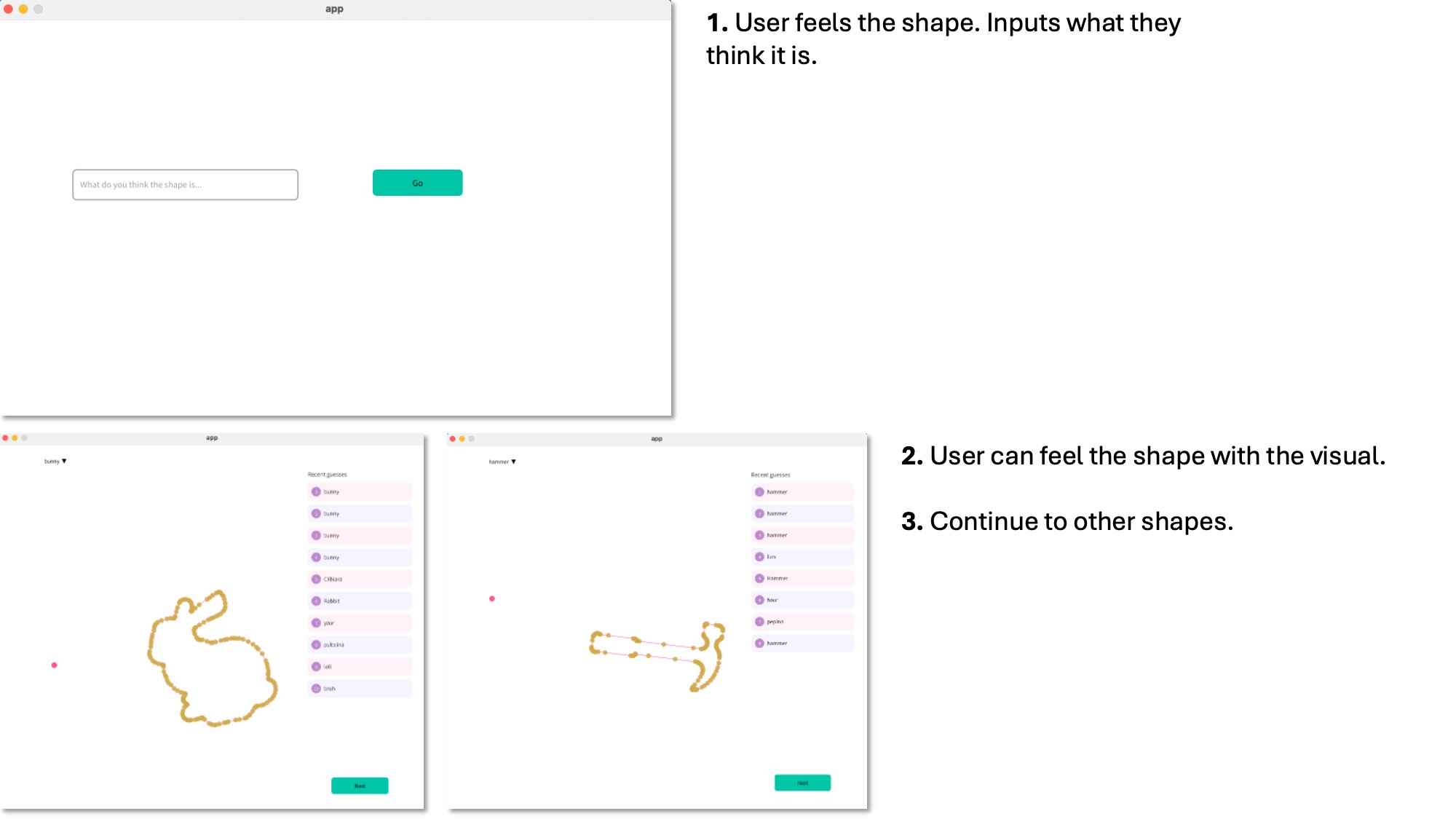
Fig 12: UI showing 1) Screen showing a blue dot as the user's cursor which is their only visual cue besides the kinesthetic feedback to guess the shape 2) User typing their response 3) Result revealed alongside previous guesses. User can now have the full visual cue as they trace the shape.
Offline shape preparation. Shapes start as SVG outlines. A Python preprocessing script (ImageProcessing.py) reads the SVG and outputs a list of 20 (x, y) boundary points that forms a closed polygon boundary in counter-clockwise order, normalized to the device�s workspace in meters. We chose the shapes of a duck, bell, banana, fish, horseshoe, and a mushroom, which were chosen and drawn for their distinguishing geometric features and also allowed for a variety of textures rendered by varying stiffness and damping coefficients. The script weights its sampling by local curvature so that sharp corners receive more points than straight segments. The script outputs a .csv file for the Processing UI, and a C array (PROGMEM) that we paste into the Arduino firmware.
SQLite database. A local SQLite database (main.db) holds two tables: ShapesTable (one row per shape, with name and CSV filename) and GuessesTable (one row per participant guess, with shape ID and timestamp). All database access goes through a small Processing module (db_comms.pde) that insert a guess, load recent guesses for a shape, get a single shape�s metadata, and list all available shapes.
Runtime visual. The Processing sketch reads xh, yh, Fx, Fy from the Arduino firmware over serial at 115200 baud and alternates between two screens. On the guess screen, only a small dot tracking the pen tip is shown, and the shape outline is hidden so the participant identifies the shape from touch alone. A text input and �Go� button submit a guess, which is written to the database. The results screen then reveals the shape outline (loaded from the CSV) alongside the dot, plus a sidebar of recent guesses. Clicking �Next� proceeds to the next shape and sends a single-character command over serial that tells the firmware which PROGMEM array to make active.
3.4 Demonstration / Application
Before interacting with the main shape-guessing game, participants are given a chance to interact with a �training� environment. In the training environment, participants are provided visual feedback to get accustomed to interacting with a position-tracking haptic system. More importantly, participants are given the opportunity to feel what each of the different textures feel like on squares of different rendered materials, before having to interact with more complex shapes. Each material is labeled as �[high/low] stiffness� and �[high/low] damping.� Once participants had a chance to feel each material texture, they would be ushered over to the other pantograph setup to interact with the main game.
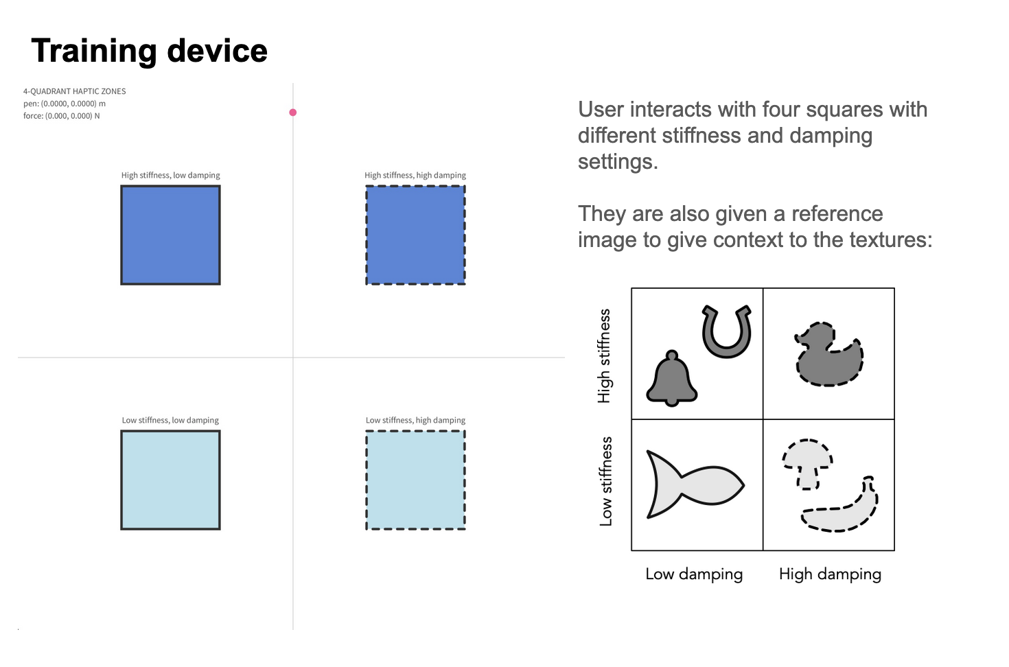
Figure 13: Training demo screen (left) + reference shapes with texture as hints (right)
Upon sitting down, users are presented with a cursor on a blank screen. By moving the pantograph, they can feel the shape of the unknown object, with the position of the cursor (proxy) providing additional visual feedback. The participants were also provided a �menu� of the 6 possible shapes that they could be encountering. The shapes were assigned to their material properties based on their real life counterparts�for example, a fish is soft and slippery, so it is rendered with low stiffness and low damping. Once the participant is sufficiently confident with their guess, they type it into the box for our data collection, then are shown the true shape they just felt. The process repeats for another one or two shapes.

Figure 14: Game instructions and sequence
Video 1: Game demo
Video 2: Test mode of all shapes rendering
4. Results
4.1 Survey responses on quality of haptic feedback
During the Open House, we provided a short survey to gather participant feedback on the perceived quality of the haptic rendering. Among the seven randomly assigned shapes presented at the demo, participants rated three metrics on a 1-5 scale as well as one binary metric:
- Noticeability: the haptic effect is clearly noticeable; there is an obvious difference in haptic feedback as the handle is moved.
- Stability and noise-freeness: the haptic effect should not feel �active� or unnaturally noisy
- Realism: outside of noise and stability, does the underlying haptic effect feel realistic?
- Funness: a binary metric (It was fun or not).
Twenty participants responded (n = 20). Results are summarized below.
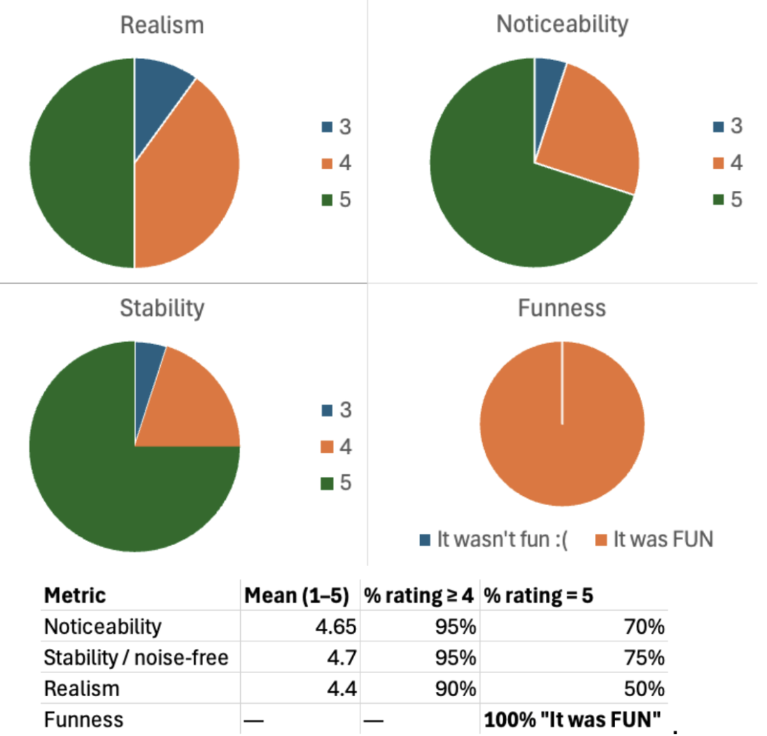
Figure 15: Results of realism, noticeability, stability, and funness
Stability scored highest (mean 4.70). This may be attributed to our fine tuning of the force commutation method using a proxy-based method, where the force is calculated between the pen and a proxy point constrained to slide along the polygon boundary, which produces a well-defined and smoothly-varying force direction even at sharp corners. Noticeability scored similarly (mean 4.65). The K = 30-50 N/m range used across the 7 shapes produced perceptible boundary contact for all shapes without causing instability while also being haptically noticeable. The damping coefficient (B = 0 or 0.03 N�s/m) was small enough not to interfere with noticing and detecting the wall itself.
Realism scored lowest (mean 4.40, with two participants rated 3) but still 90% rated it 4 or 5. The rendered stiffness was capped at K = 50 N/m across all shapes since we�ve tested that higher stiffness caused instability. As a result, the wall may still feel squishy and not as hard as a real surface on which the user can also push the pen far enough through the shape that the proxy jumps from one boundary segment to another rather than tracking the original contact point. This changes the felt force direction and reduces the realism. Additionally, identifying objects through kinesthetic feedback using a 2D point contact is an unfamiliar perceptual task, because humans normally explore objects using both kinesthetic and tactile feedback with multiple fingers in 3D. Thus, even with perfect rendering, the experience may feel somewhat unlike touching a real shape.
All 20 respondents selected �It was FUN�, consistent with visitors at the demo attempting multiple trials on multiple shapes.
4.2 Shape recognition performance
We logged 70 interpretable shape guesses across the open house, of which 52 were correct, giving an overall shape recognition accuracy of 74.3%, which is well above the 14.3% expected from random guessing across 7 shapes. Per-shape accuracy varied: duck (87.5%), fish (79.4%), horseshoe (80.0%), and square (80.0%) were identified most reliably, while bell (40.0%) and banana (60.0%) were the hardest.
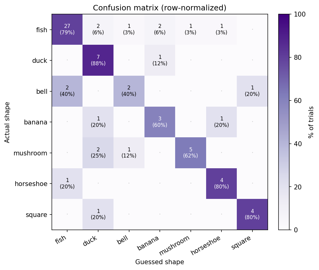
Figure 16: Confusion matrix showing actual shape vs. guessed shape
The confusion matrix shows the most common confusions were fish guessed as duck or banana and mushroom guessed as duck, while the bell was most often misidentified as fish, possibly because of rounded features in the shape (e.g. lower half of the fish and banana) feel similar to other rounded outlines without visual reference. These results should be interpreted as preliminary: trial counts were small and not entirely balanced (fish was rendered 34 times due to being the default startup shape, others only 5-8 times each). Overall, participants were able to use the device to recognize shapes accurately, above the probability expected from random guessing.
5. Future Work
On the hardware side, the most immediate improvement would be reducing the residual friction and inertia of the linkage so free space feels closer to truly free. The joint friction noted in Section 3.1 came from the trade-off between overtightening and undertightening the press-fit screw joints; replacing these with proper bearings on every axis would likely give a much more transparent device. Stronger motors would also let us increase the stiffness from K = 50 N/m without running into PWM saturation and stability issues, which would make the boundary feel sharper and reduce how often the proxy jumps to a different segment when the user pushes into a shape. Increasing the boundary coordinate resolution from 20 vertices to a higher count, or smoothing the force direction across vertices, would also make curved features smoother.
On the experimental study side, a natural next step is to run a controlled study where each participant tries the same set of shapes both with and without stiffness and damping cues, recording guess accuracy and exploration time for each condition. A similar comparison could be set up for fine textures: rendering the same outlines with and without a small high-frequency vibration simulating fine texture along the boundary, and measuring whether the added texture cue improves recognition. These two comparisons together would let us isolate the contribution of each type of feedback and more directly determine the effect of haptic cues in shape identification.
6. Acknowledgments
We would like to thank Megan Coram, Elizabeth Childs, and Xinyi Liang for their constant support throughout the course, and Dr. Allison Okamura for teaching ME327 and providing invaluable guidance and mentorship. We also thank the 2025 Group 12 team for inspiring our pantograph design and implementation.
7. Files
Visit the GitHub for the entire codebase: https://github.com/chiarac99/2DShapeRenderingPantograph
8. References
[1] G. Campion, Q. Wang, and V. Hayward, (2005) The Pantograph Mk-II: A Haptic Instrument. Proc. IEEE/RSJ Int. Conf. Intelligent Robots and Systems (IROS), Edmonton, Canada, pp. 723�728.
[2] D. A. Lawrence, (1992) Stability and transparency in bilateral teleoperation. Proc. of the 31st IEEE Conference on Decision and Control, Tucson, AZ, USA, 1992, pp. 2649-2655 vol.3
[3] Hayward V, Astley OR, Cruz; Hernandez M, Grant D, Robles; De La Torre G (2004), Haptic interfaces and devices. Sensor Review, Vol. 24 No. 1 pp. 16�29
[4] Ratschat AL, van Rooij BM, Luijten J and Marchal-Crespo L (2024) Evaluating tactile feedback in addition to kinesthetic feedback for haptic shape rendering: a pilot study. Front. Robot. AI 11:1298537
[5] Klatzky, R. L., Lederman, S. J., & Reed, C. (1987). There's more to touch than meets the eye: The salience of object attributes for haptics with and without vision. Journal of Experimental Psychology: General, 116(4), pp. 356�369
[6] Norman, J.F., Bartholomew, A.N. (2011) Blindness enhances tactile acuity and haptic 3-D shape discrimination. Atten Percept Psychophys 73, pp. 2323�2331
[7] Susan J Lederman, Roberta L Klatzky, (1987) Hand movements: A window into haptic object recognition. Cognitive Psychology 19(3) pp. 342-368
[8] Ottink, L., van Raalte, B., Doeller, C.F. et al. (2022) Cognitive map formation through tactile map navigation in visually impaired and sighted persons. Sci Rep 12, pp. 11567
[9] S. Choi and H. Z. Tan, (2004) Toward realistic haptic rendering of surface textures. IEEE Computer Graphics and Applications, vol. 24, no. 2, pp. 40-47
[10] Chen, S.; Yuan, T.; Xu, L.; Ru, W.; Wang, D. (2025) A systematic review of haptic texture reproduction technology. Intell. Robot. , 5(3), pp. 607-30
[11] Kumari, P., Chaudhuri, S., (2016), Haptic Rendering of Thin, Deformable Objects with Spatially Varying Stiffness. Haptics: Perception, Devices, Control, and Applications. EuroHaptics. Lecture Notes in Computer Science, vol 9774
[12] D. J. Brewer, D. J. Meyer, M. A. Peshkin and J. E. Colgate, (2016) Viscous textures: Velocity dependence in fingertip-surface scanning interaction. IEEE Haptics Symposium (HAPTICS), Philadelphia, PA, USA, pp. 265-270
[13] S. Choi and H. Z. Tan, (2004) "Perceived Instability of Virtual Haptic Texture. I. Experimental Studies," in Presence, vol. 13, no. 4, pp. 395-415
9. Appendix: Project Checkpoints
9.1 Checkpoint 1
Our goals for Checkpoint 1 were to (i) complete design of the mechanical system (including motor and encoder selection); and (ii) produce a detailed plan of haptic rendering algorithms and controls.
Design of mechanical system
Pantograph design
We designed a four-linkage pantograph inspired by previous ME327 projects that utilize two Hapkits. We decided to fully redesign the sector pulleys and have an overlapping axis for the center rotation of the sectors. The pantograph handle resembles a pen with two axes for rotation that will allow users to get a comfortable grip and simulate a real "drawing" experience. To achieve this, we created a rotating fifth linkage, shown in the image below as the dark orange link. We 3D printed the linkages in PETG using an Ender 3D Printer. Then, to ensure that free space feels truly free, we press-fit solid metal bushings on each of the linkages' ends and used shoulder screws to ensure there was no friction while rotating. The other end of the linkage was intentionally left to be hand-tapped to secure the screw with no additional nuts. The base was designed as well, completing checkpoint 1 and is in the process of being 3D printed with a Bambu printer in PLA filament. The base has spaces to fit five rubber suction cups, and near the motors, it has holes where zipties will secure the motors in place. This part is printed in two parts to reduce the number of supports needed.
Encoders and motor selection
We first planned to use the Maxon RE-max motors because they have 8x more torque than the Mabuchi Hapkit motors at 5V, but the Maxons� stall current at 5V is higher than the motor driver of the Hapkit board can handle (2A max for the L298P). There were some work arounds that we thought of: 1) limit the voltage applied to 2.10V, and it would still have like 3x more torque than the Hapkit motor, or 2) use Polulu motor drivers to allow for higher voltages and higher torques. For the first solution, there's no safe way to limit current with the Hapkit's motor driver, so we could have run into overheating issues. Additionally, when designing the base for the pantograph, the motors are quite heavy and need to go at the bottom of the base. This complicated the design for the capstans, so we ultimately decided to proceed with the Hapkit motors and the magnetic encoder that comes with the Hapkit board.
Kinematics & Controls
Haptic Rendering Architecture
The block diagram below shows how the three main parts of the system are connected in a closed loop. The user moves the pen tip, the firmware reads the resulting encoder angles and computes a force command, the motors actuate to deliver that command back to the user, and the same pen-tip position is sent over serial to the visual interface.
Please reference the 5-bar linkage below for the variables shown in the block diagram above.
Direct Kinematics
To render force feedback in the correct direction and at the correct location, the firmware needs to know where the pen tip is in 2D Cartesian space at each loop iteration. The only sensors available are the two motor encoders at the base, so we use forward kinematics to map the two measured joint angles (θ₁, θ₅) to the end-effector position P₃ = (x₃, y₃). See figure below for a general 5-bar linkage [1].
Our linkage is a modified five-bar pantograph with the two motors placed at the same x-y location (a₅ = 0), which gives us a wider horizontal workspace than the standard configuration. Following the geometric approach of Campion et al. [1], we treat P₃ as the tip of the triangle P₂P₃P₄, where P₂ and P₄ are the elbows directly driven by the two motors. The derivation proceeds in the following steps:
- Compute the elbow positions P₂ and P₄ directly from θ₁ and θ₅, since each elbow lies at the end of a link directly connected to the motor.
- Find the distance between P₂ and Pₕ using the right triangles P₂PₕP₃ and P₄PₕP₃.
- Compute the altitude ‖P₃ − Pₕ‖ by the Pythagorean theorem.
- Find the coordinates of the base of the height (Pₕ) from P₃ that's on the segment connecting P₂ and P₄.
- Step perpendicular to P₂P₄ from Pₕ by that altitude, choosing the sign convention that places P₃ in the "elbow up" half-plane (the configuration the device actually operates in).
The full derivation, including the resulting closed-form expressions for x₃ and y₃ in terms of θ₁ and θ₅, is shown below.
With this forward-kinematics model, given a sensor reading on each loop, the firmware can compute the pen tip's (x, y) position in real time, which is needed for the force-feedback rendering described in the later sections.
Differential Kinematics
Forward kinematics gives us where the pen tip is. To turn the desired force from the force-feedback model into commands the motors can execute, we need the Jacobian. The Jacobian relates joint-angle changes to end-effector displacement, and its transpose maps a Cartesian force at the pen tip to the two motor torques required to produce it: τ = Jᵀ � F_world. This is the step that closes the loop from the force-feedback model back to the actuators.
Because x₃ and y₃ are built up through a chain of intermediate quantities (P₂, P₄, d = ‖P₂ − P₄‖, b = ‖P₂ − Pₕ‖, h = ‖P₃ − Pₕ‖, Pₕ), the partial derivatives ∂x₃/∂θᵢ and ∂y₃/∂θᵢ are computed by the chain rule applied through each of those intermediate quantities in the same order as the forward-kinematics derivation. We follow the chain-rule expressions in Campion et al. [1]; the Jacobian and its set of equations are shown below.
Once the Jacobian is evaluated at the current configuration, the torque required from each motor to render a force F_world = (Fₓ, F_y) at the pen tip would be τ = Jᵀ � F_world. Each Hapkit board then converts its torque to a motor PWM command using the transmission mechanism relation (Tₚ = F � rₕ � rₚ / rₛ) we used in the homework assignments. This completes the sensors-to-actuation loop: encoder reading → forward kinematics → pen-tip position → [force-feedback model] → F_world → Jᵀ → motor torques → PWM → motor command.
Force Feedback Model
For force feedback, we need to convert an image to a series of points that can be used by the microcontroller to check whether the user has penetrated into the shape. Once the penetration depth is known, then force feedback can be calculated with the appropriate direction. The diagram below describes the rendering pipeline from getting from an SVG file through to providing force feedback to the user. Currently, our three demo objects will be the Stanford bunny, a hammer, and a pear.
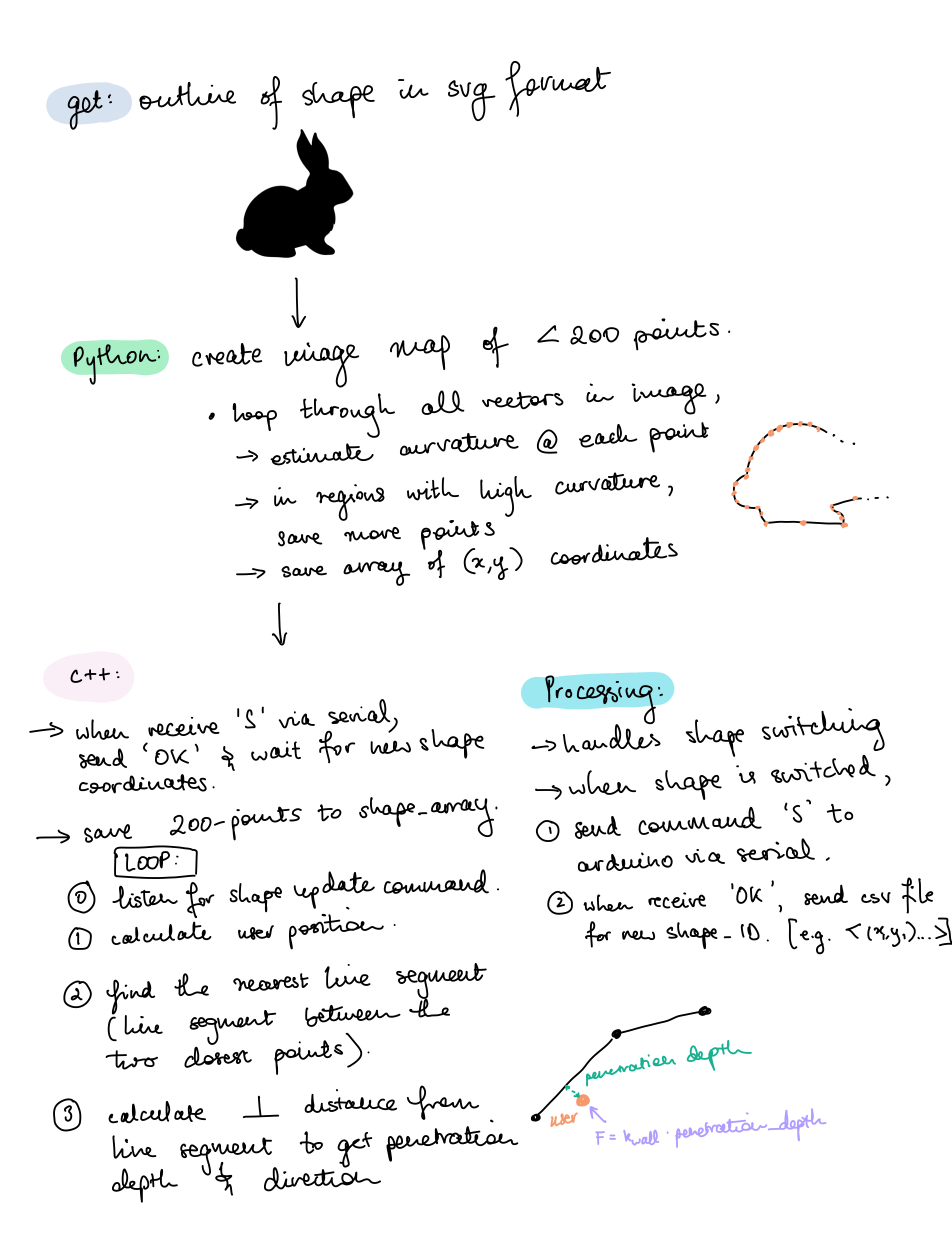
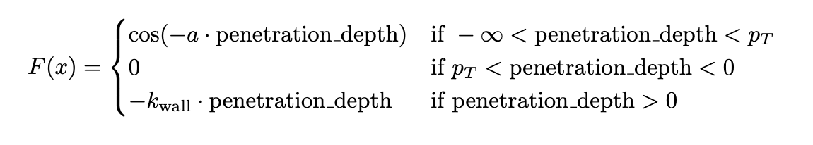
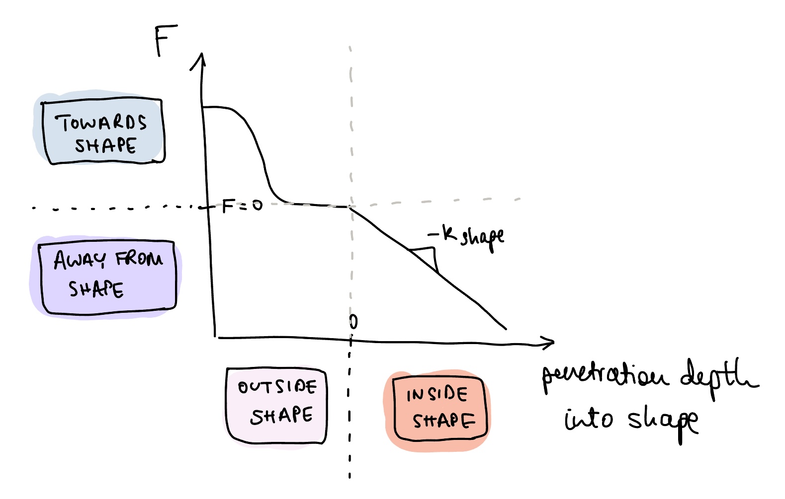
Now that we have penetration depth and penetration direction, we need to understand how force changes over penetration depth. The graph below shows a gradual slope into the region where the shape is located. Then, a force away from the shape is applied once the user has crossed into the shape. We also define equations for this force where p_T is some penetration depth threshold where we want the user to sit in free space, just outside the shape.
Note: These shapes might feel super discrete. The problem is that for every loop on the microcontroller, we will need to calculate the user's distance from every point in the map. This week, we plan to look into other methods of determining the user's distance from the closest line.
As a final note, we are also considering adding damping or arc-length dependent sinusoidal vibrations to simulate high friction versus low friction surfaces or 'fuzziness' of an object. This will have to be tested with the built pantograph to see if it adds value to object classification.
Graphics
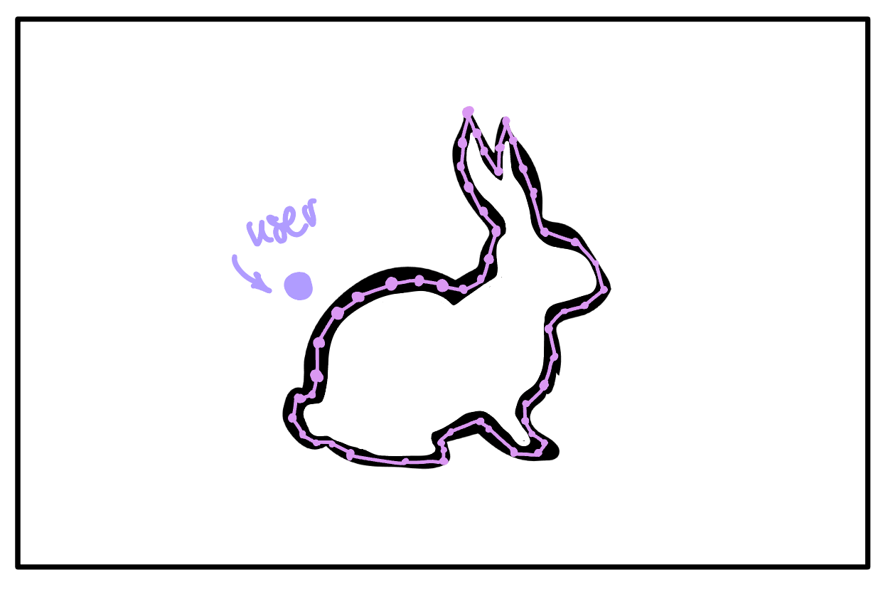
Graphics will be necessary for testing. Black lines from adjacent points in the shape map should be overlaid on the original SVG, and the user's position should be indicated by a small circle (as shown below).
We write a simple UI with database integration on Processing. The flow between these two parts of the system is shown below. We will have an option in the interface to move between shapes. There will be six total shape options, two for each shape: one version will be our controlled group that has no stiffness or textural feedback and the second will have stiffness and textural feedback.
9.2 Checkpoint 2
Goals met:
- Hardware is complete.

- Simulation of penetration depth and force feedback models done on Processing.

- Arduino code with penetration depth and haptic feedback calculations is complete and is currently being debugged.
- Processing UI and communications with arduino are complete.
- Integration with software and hardware is in progress.
All software is available on the github: [[https://github.com/chiarac99/2DShapeRenderingPantograph ]]
Some challenges that were encountered were:
- The usb serial and power supply ports were not accessible on the second board because of interference with the other board. But cutting some unused pins off the first board and finding a thinner cable, we were able to get them both attached.
- The slot were the screw is pushed through to secure the motor is thinner than the Hapkit. Tightening the screw has caused a little interference with the capstan, which adds friction to the assembly.
- During integration, it was recognised that both boards needed to be connected to the computer and the current method for changing the shape being rendered was did not account for multiple boards. The Processing code was adapted for two serial ports instead of one.